

Abstract
The physiological role of a-synuclein (a-syn), an intrinsically disordered presynaptic neuronal protein, is believed to impact the release of neurotransmitters through interactions with the SNARE complex. However, under certain cellular conditions that are not well understood, a-syn will self-assemble into β-sheet-rich fibrils that accumulate and form insoluble neuronal inclusions. Studies of patient-derived brain tissues have concluded that these inclusions are associated with Parkinson’s disease, the second most common neurodegenerative disorder, and other synuclein-related diseases called synucleinopathies. In addition, repetitions of specific mutations to the SNCA gene, the gene that encodes a-syn, result in an increased disposition for synucleinopathies. The latest advances in cryo-EM structure determination and real-space helical reconstruction methods have resulted in over 60 in vitro structures of a-syn fibrils solved to date, with a handful of these reaching a resolution below 2.5 Å. Here, we provide a protocol for a-syn protein expression, purification, and fibrilization. We detail how sample quality is assessed by negative stain transmission electron microscopy (NS-TEM) analysis and followed by sample vitrification using the Vitrobot Mark IV vitrification robot. We provide a detailed step-by-step protocol for high-resolution cryo-EM structure determination of a-syn fibrils using RELION and a series of specialized helical reconstruction tools that can be run within RELION. Finally, we detail how ChimeraX, Coot, and Phenix are used to build and refine a molecular model into the high-resolution cryo-EM map. This workflow resulted in a 2.04 Å structure of a-syn fibrils with excellent resolution of residues 36–97 and an additional island of density for residues 15–22 that had not been previously reported. This workflow should serve as a starting point for individuals new to the neurodegeneration and structural biology fields. Together, this procedure lays the foundation for advanced structural studies of a-syn and other amyloid fibrils.
Key features
• In vitro fibril amplification method yielding twisting fibrils that span several micrometers in length and are suitable for cryo-EM structure determination.
• High-throughput cryo-EM data collection of neurodegenerative fibrils, such as alpha-synuclein.
• Use of RELION implementations of helical reconstruction algorithms to generate high-resolution 3D structures of a-synuclein fibrils.
• Brief demonstration of the use of ChimeraX, Coot, and Phenix for molecular model building and refinement.
Keywords: Cryo-EM, Helical reconstruction, Alpha-synuclein, Amyloid proteins, Neurodegeneration, Vitrification
Graphical overview
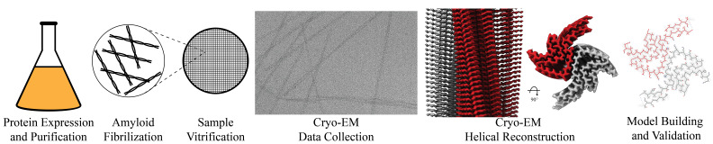
Graphical overview of a-synuclein fibrilization and cryo-EM structure determination. a-syn protein expression and purification is followed by a fibrilization protocol yielding twisting filaments that span several micrometers in length and are validated by negative stain transmission electron microscopy (NS-TEM). The sample is then vitrified, followed by cryo-EM data collection. Real-space helical reconstruction is performed in RELION to generate an electron potential map that is used for model building.
Background
Amyloid formation within neurons has been well documented to cause neurodegeneration in patients leading to a variety of diseases including Alzheimer’s (AH), Parkinson’s disease (PD), Lewy Body disease (LB), and multiple system atrophy (MSA) [1–3]. The formation of amyloids is due to protein aggregation resulting in helical, filamentous assemblies with cross β-sheet quaternary structure (Figure 1) [4]. Amyloid filaments interact with different cellular components such as membranes, cytoskeletal factors, and other filaments to form inclusion bodies that disrupt cellular processes and ultimately lead to cell death [2]. These inclusion bodies are prominent in the postmortem brains of patients who have suffered from these neurodegenerative diseases, and early investigation of inclusion bodies revealed the presence of filamentous a-synuclein (a-syn) [1,2]. a-syn is a small (14.4 kDa) intrinsically disordered protein whose physiological role remains elusive. a-syn has the capability to bind to the SNARE complex and associate with vesicles at the neuronal axon terminus, providing evidence that it may have an impact on neurotransmitter release, vesicle docking, and vesicle trafficking [5–8]. However, upon misfolding, a-syn first forms oligomeric aggregates that eventually undergo fibrilization; these fibrils display the highly ordered cross β-sheets classically found in amyloids [9,10]. These, in turn, form the extended filaments that cause neuropathological changes in the brain and are specifically responsible for PD, LB, and MSA. Diseases caused by a-syn in this manner are called synucleinopathies [11].
Figure 1. Structural features of a-syn fibrils from cryo-EM structures.

A. Cryo-EM structure of full-length a-syn fibril depicting two protofilaments (one in red; one in grey). B. Magnified view of a-syn fibril portraying stacked rungs and filament twist. C. Cross-section of a-syn fibril electron potential map displaying two a-syn monomers that comprise each protofilament, approximately 180° from each other. D. Electron potential map of individual β-sheet stacks twisting. E. Model depicting the secondary structure of stacking β-sheets. F. Example of rise measurement for P21 symmetry (red) and C2 symmetry (blue). G. Possible packing symmetry between protofilaments for P21 symmetry (out of register) (red) and C2 symmetry (in register) (blue).
The high-resolution structure presented here of filamentous wild-type a-syn is of a helical filament composed of two protofilaments; each turn (or rung) of the filament is comprised of two copies (one per protofilament) of a-syn facing nearly 180° from each other (Figure 1). Between the monomers that make up each protofilament, there is a hydrophobic interface composed of residues 50–57, similar to previously solved structures of filamentous a-syn [12–14]. This interface is stabilized by salt bridges and pseudo-screw symmetry, as previously reported [12,13]. For a-syn, there are seven different missense familial mutations commonly found in patients who have a higher disposition for synucleinopathies (A30P, E46K, H50Q, G51D, A53E, A53T, and A53V) [15–21]. Interestingly, six of these familial mutations lie within the core of the structure and may cause destabilization, resulting in a variety of different fibril morphologies. The presence of polymorphism has been demonstrated particularly well through the analysis of in vitro a-syn fibrils. Fibril twist, crossover distance, packing arrangement, number of protofilaments, interface, and tertiary structure, among others, can vary greatly under different micro- and macro-environments. Many different environmental factors such as pH, salt concentration, temperature, quiescence, and post-translational modifications have an impact on fibril morphology. This has led to the documentation of more than 60 in vitro structural polymorphs of a-syn in the PDB [22,23]. These structural differences in the in vitro filaments can have direct effects on nucleation rates, seeding propensities, and even cytotoxicity [23]. Unfortunately, the ties between these structurally distinct in vitro polymorphs to those found in sarkosyl-insoluble brain-derived structures remain elusive. However, evidence suggests that different polymorphs may influence pathologies [24–26]. This is demonstrated by the difference in a-syn folds of the filaments extracted from patients diagnosed with MSA vs. PD [27].
The formation of the filaments responsible for synucleinopathies is propagated in brain tissue by primary nucleation events in which a-syn monomer spontaneously undergoes structural changes resulting in nucleation. This nucleation site can then recruit additional a-syn monomers to bind, thus elongating the fibril [28,29]. However, there can also be secondary nucleation events in which preformed fibrils are introduced into the cellular environment as “seeds” [30]. These seeding events are significantly more potent at fibril formation and elongation. Remarkably, seeds from a particular polymorph have been shown to recruit wild-type a-syn, provide a structural template, and form filaments expressing the polymorph of the seed regardless of whether the endogenous protein recruited is pathogenic or not [31]. A consequence of this prion-like self-replication is that a-syn fibrils may move from cell to cell, spreading cytotoxic polymorphs.
The introduction of polymorphism has a multifactorial effect on clinical treatments of neurodegenerative diseases. Our understanding of the implications associated with each polymorph on disease progression, pathology, and patient outcomes is very limited. In addition, the differences in folding, packing, or twists of each polymorph introduce complexities in binding sites, affinities, and accessibility for a “one size fits all” drug for synucleinopathies. This is further complicated by evidence that not only are there disease-specific morphisms but each synucleinopathy can exhibit patient-to-patient heterogeneity [32]. Thus, to overcome these challenges, explore new therapeutic targets, understand specific polymorph effects on neuropathology, and develop therapies with patient-specific approaches, solving both patient-derived and in vitro amyloid polymorphs should be explored.
Here, we describe a helical reconstruction workflow that we use to solve the structure of in vitro assembled filamentous a-syn to a global resolution of 2.04 Å. We purify a-syn filaments from a reaction in which fibril seeding material is combined with monomeric a-syn. The fibril seeding material provides a template for fibril elongation via monomer addition over a 6-week incubation period at 37 °C with shaking at 250 rpm. The purified a-syn filaments are then imaged using negative stain transmission electron microscopy (NS-TEM) to evaluate sample integrity and fibril concentration on the grid. The sample is then applied to grids and plunge frozen, and the vitrified grids are used for cryo-EM data collection. We provide a detailed protocol utilizing RELION to reconstruct a high-resolution cryo-EM electron potential map that is then used for building an atomic model of the fibril (Figure 1B, 1C, 1E). The steps presented here may be applied to studies of various amyloid fibrils and accelerate cryo-EM structure determination in the fields of neurodegenerative research and medicine.
Materials and reagents
Biological materials
1. Plasmid with wild-type a-syn construct in E. coli BL21(DE3)/pET28a-AS [33]
Reagents
1. LB broth (Invitrogen, catalog number: 12780029)
2. Bacto agar (Dot Scientific Inc., catalog number: DSA20030-1000)
3. Magnesium sulfate (MgSO4) (Fisher Scientific, catalog number: 01-337-186)
4. Calcium chloride (CaCl2) (Fisher Scientific, catalog number: BP510-500)
5. Sodium phosphate (NaH2PO4) (Fisher Scientific, catalog number: 01-337-702)
6. Potassium phosphate (KH2PO4) (Fisher Scientific, catalog number: 01-337-803)
7. Sodium chloride (NaCl) (Fisher Scientific, catalog number: S271-500)
8. IPTG (Fisher Scientific, catalog number: BP1755-10)
9. Tris-HCl (Fisher Scientific, catalog number: PRH5125)
10. EDTA (Fisher Scientific, catalog number: AAA1516130)
11. Kanamycin monosulfate (Thermo Scientific, catalog number: J61272.14)
12. SDS-PAGE gels (Bio-Rad, catalog number: 4561096)
13. SDS-PAGE loading dye (Bio-Rad, catalog number: 1610737)
14. Coomassie Brilliant Blue (TCI, catalog number: 6104-59-2)
15. BME vitamins (Sigma-Aldrich, catalog number: B6891-100mL)
16. Sodium azide (Sigma-Aldrich, catalog number: 19-993-1)
17. Studier trace metal mix (Sigma-Aldrich, catalog number: 41106212)
18. Ammonium sulfate (Fisher Scientific, catalog number: A702-500)
19. Deuterium oxide (2H2O) (Cambridge Isotopes Laboratories, catalog number: DLM-4-1L)
20. BioExpress bacterial cell media 10× concentrate (U-13C, 98%; U-15N, 98%; U-D 98%) (Cambridge Isotopes Laboratories, catalog number: CGM-1000-CDN)
21. 15N-NH4CI (Cambridge Isotopes Laboratories, catalog number: 39466-62-10)
22. 2H-13C-glucose (Cambridge Isotopes Laboratories, catalog number: CDLM-3813-5)
23. Sodium deuteroxide (NaO2H) (Cambridge Isotopes Laboratories, catalog number: DLM-45-100)
24. 2% uranyl acetate (UA) (EMS, catalog number: 22400-2)
25. Ethane (C2H6) (Airgas, catalog number: ET RP35)
26. Liquid nitrogen (LN2) (Airgas, catalog number: NI UHP230LT350)
Solutions
1. Kanamycin stock solution, 1,000× (40 mg/mL) (see Recipes)
2. Kanamycin stock solution, 1,000× (90 mg/mL) (see Recipes)
3. Conditioning plate (see Recipes)
4. Pre-growth media (see Recipes)
5. Lysis buffer (see Recipes)
6. Wash buffer (see Recipes)
7. Growth media (see Recipes)
8. IPTG stock solution (see Recipes)
9. Buffer A (see Recipes)
10. Buffer B (see Recipes)
11. TEN buffer (see Recipes)
12. Saturated ammonium sulfate solution (see Recipes)
13. Fibrilization buffer (see Recipes)
14. 1% uranyl acetate (UA) (see Recipes)
Recipes
1. Kanamycin stock solution, 1,000× (40 mg/mL)
| Reagent | Final concentration | Amount |
|---|---|---|
| Kanamycin monosulfate | 40 mg/mL | 0.4 g |
| 2H2O | n/a | 10 mL |
| Total | n/a | 10 mL |
a. Completely dissolve kanamycin monosulfate in 2H2O.
b. Sterilize solution using a 0.22 μm syringe filter and 10 mL syringe.
c. Aliquot 1,000 μL stocks and store at -20 °C until use.
2. Kanamycin stock solution, 1,000× (90 mg/mL)
| Reagent | Final concentration | Amount |
|---|---|---|
| Kanamycin monosulfate | 90 mg/mL | 0.9 g |
| 2H2O | n/a | 10 mL |
| Total | n/a | 10 mL |
a. Completely dissolve kanamycin monosulfate in 2H2O.
b. Sterilize solution using a 0.22 μm syringe filter and 10 mL syringe.
c. Aliquot 1,000 μL stocks and store at -20 °C until use.
3. Conditioning plate
| Reagent | Final concentration | Amount |
|---|---|---|
| 2H2O | 70% | 700 mL |
| LB broth | 2% | 20 g |
| Bacto agar | 1.5% | 15 g |
| H2O | n/a | Fill to 1,000 mL |
| Total | n/a | 1,000 mL |
a. Combine reagents in a flask and autoclave at 121 °C, 15 psi for at least 20 min.
b. Allow the media to cool to ~55 °C, then add 1,000 μL of the kanamycin stock solution (1,000×, 40 mg/mL).
c. Pour ~25 mL of media per Petri plate (100 mm) and repeat for the remaining 1 L.
4. Pre-growth media
| Reagent | Final concentration | Amount |
|---|---|---|
| 2H2O | 70% | 35 mL |
| LB broth | 2% | 1 g |
| H2O | n/a | Fill to 50 mL |
| Total | n/a | 50 mL |
a. Combine reagents in a flask and autoclave at 121 °C, 15 psi for at least 20 min.
b. Allow the media to cool to ~55 °C and then add 50 μL of the kanamycin stock solution (1,000×, 40 mg/mL).
5. Lysis buffer
| Reagent | Final concentration | Amount |
|---|---|---|
| NaOH | 40 mM | 0.80 g |
| Tris-HCl | 20 mM | 3.15 g |
| EDTA | 1 mM | 0.0585 mg |
| Triton X-100 | 0.1% (v/v) | 0.5 mL |
| Total | n/a | 500 mL |
Combine reagents and adjust pH to 8.0 with NaOH.
6. Wash buffer
| Reagent | Final concentration | Amount |
|---|---|---|
| NaH2PO4 | 50 mM | 0.34 g |
| KH2PO4 | 25 mM | 0.17 g |
| NaCl | 10 mM | 0.03 g |
| 2H2O | n/a | Fill to 50 mL |
| Total | n/a | 50 mL |
a. Combine reagents and adjust the pH to 7.6 with NaO2H.
b. Filter sterilize the solution using a 500 mL filtration system.
7. Growth media
| Reagent | Final concentration | Amount |
|---|---|---|
| NaH2PO4 | 50 mM | 6.9 g |
| KH2PO4 | 25 mM | 3.4 g |
| NaCl | 10 mM | 0.58 g |
| MgSO4 | 5 mM | 1.23 g |
| CaCl2 | 0.2 mM | 0.03 g |
| Bacterial cell media 10× | 0.1× | 10 mL |
| BME vitamins 100× | 0.25× | 2.5 mL |
| Studier trace metals 1,000× | 0.25× | 0.25 mL |
| 15N-NH4CI | 1 g/L | 1 g |
| 2H-13C-glucose | 8 g/L | 8 g |
| BME vitamins | 0.25× | 2.5 mL |
| 2H2O | n/a | Fill to 50 mL |
| Total | n/a | 1,000 mL |
a. Combine reagents and add 1,000 μL of the kanamycin stock solution (1,000×, 90 mg/mL). Adjust pH to 7.6 with NaO2H.
b. Filter sterilize the solution using a 1,000 mL filtration system.
8. IPTG stock solution
| Reagent | Final concentration | Amount |
|---|---|---|
| IPTG | 0.5 M | 1.2 g |
| 2H2O | n/a | 10 mL |
| Total | n/a | 10 mL |
a. Completely dissolve IPTG in 2H2O.
b. Sterilize solution using a 0.22 μm syringe filter and 10 mL syringe.
c. Aliquot 1,000 μL stocks and store at -20 °C until use.
9. Buffer A
| Reagent | Final concentration | Amount |
|---|---|---|
| Tris-HCl | 30 mM | 4.73 g |
| NaCl | 30 mM | 1.75 g |
| H2O | n/a | 1 L |
| Total | n/a | 1 L |
a. Dissolve Tris-HCl and NaCl in water while stirring.
b. Adjust pH to 7.4 at 37 °C using 1 M NaOH.
10. Buffer B
| Reagent | Final concentration | Amount |
|---|---|---|
| Tris-HCl | 30 mM | 2.36 g |
| NaCl | 1 M | 29.22 g |
| H2O | n/a | 500 mL |
| Total | n/a | 500 mL |
a. Dissolve Tris-HCl and NaCl in water while stirring.
b. Adjust pH to 7.4 at 37 °C using 1 M NaOH.
11. TEN buffer
| Reagent | Final concentration | Amount |
|---|---|---|
| Tris-HCl | 30 mM | 4.73 g |
| NaCl | 30 mM | 1.75 g |
| EDTA | 0.1 mM | 29.22 mg |
| H2O | n/a | 1 L |
| Total | n/a | 1 L |
a. Dissolve Tris-HCl, NaCl, and EDTA in water while stirring.
b. Adjust pH to 8.0 at 37 °C using 1 M NaOH.
12. Saturated ammonium sulfate solution
| Reagent | Final concentration | Amount |
|---|---|---|
| Ammonium sulfate | saturated | ~550 g |
| H2O | n/a | 1 L |
| Total | n/a | 1 L |
a. Add ammonium sulfate into water while stirring.
b. Heat gently until all ammonium sulfate is dissolved.
c. Cool to room temperature. Crystals should form to indicate the solution is saturated.
13. Fibrilization buffer
| Reagent | Final concentration | Amount |
|---|---|---|
| NaH2PO4 | 50 mM | 1.2 g |
| EDTA | 0.1 mM | 5.85 mg |
| Sodium azide | 0.02% | 40 µg |
| H2O | 20% | 40 mL |
| 2H2O | 80% | 160 mL |
| Total | n/a | 200 mL |
a. Add NaH2PO4, EDTA, and 0.02% sodium azide solution into 2H2O and H2O.
b. Adjust pH to 7.4 at 37 °C using 1M NaO2H.
14. 1% uranyl acetate (UA)
| Reagent | Final concentration | Amount |
|---|---|---|
| 2% uranyl acetate | 1% (v/v) | 250 μL |
| H2O | n/a | 250 μL |
| Total | n/a | 500 μL |
Mix 1 part of sterile water with 1 part of 2% UA and filter through a Spin-X centrifuge tube with a 0.22 μm filter.
Laboratory supplies
1. 10 mL syringe (BD, catalog number: 309604)
2. 0.22 μm filter (GenClone, catalog number: 25-240)
3. 100 mm × 15 mm Petri dishes (Fisher Scientific, catalog number: S33580A)
4. 500 mL filtration system (Nalgene, catalog number: 595-4520)
5. 1,000 mL filtration system (Fisher Scientific, catalog number: FB12566506)
6. 50 mL conical tubes (VWR, catalog number: 525-1074)
7. 0.45 μm syringe filter (GenClone, catalog number: 25-246)
8. 1.7 mL centrifuge tubes (Denville, catalog number: C2170)
9. Parafilm (Bemis, catalog number: PM996)
10. 0.22 μm Spin-X centrifuge tube filter (Costar, catalog number: 8160)
11. 200 mesh carbon film, copper grids (EMS, catalog number: CF200-CU)
12. Whatman #1 filter paper (Whatman, catalog number: 1001-090)
13. Quantifoil R2/1 200 mesh, copper grids (Quantifoil Micro Tools GmbH, catalog number: Q210CR1)
14. Standard Vitrobot filter paper, Ø 55/20 mm, grade 595 (Ted Pella, catalog number: 47000-100)
Equipment
1. HiTrap Q HP anion exchange column with QFF anion exchange resin (Cytiva, catalog number: 17115401)
2. Stirred cell concentrator (Amicon, catalog number: UFSC05001)
3. Ultracel 3 kDa ultrafiltration disc (Amicon, catalog number: PLBC04310)
4. HiPrep 16/60 Sephacryl S100-HR gel filtration column (Cytiva, catalog number: 17119501)
5. 5424 R microcentrifuge (Eppendorf, catalog number: 05-400-005)
6. 5810 R centrifuge (Eppendorf, catalog number: 022625101)
7. J6-MI high-capacity centrifuge (Beckman Coulter, catalog number: 449598)
8. 1 L centrifuge bottle (Beckman Coulter, catalog number: C31597)
9. myTemp digital incubator (Benchmark Scientific, catalog number: H2200-HC)
10. Pyrex 250 mL Erlenmeyer flask (Corning, catalog number: 4980-250)
11. Floor orbital shaker (Thermo Electron Corporation, catalog number: 19141, model: 480)
12. Denovix UV spectrophotometer/fluorimeter (Denovix, model: DS-11 FX+)
13. Quartz cuvette (Denovix, catalog number: A-70031)
14. ӒKTA pure 25 M (Cytiva, catalog number: 29018226)
15. Grid holder block (Pelco, catalog number: 16820-25)
16. Plasma cleaner (Harrick Plasma Inc., catalog number: PDC-32G)
17. Static dissipator (Mettler Toledo, catalog number: UX-11337-99)
18. Style N5 reverse pressure tweezers (Dumont, catalog number: 0202-N5-PS-1)
19. Talos L120C 120 kV transmission electron microscope (TEM) (Thermo Fisher Scientific or equivalent)
20. Cryo grid box (Sub-Angstrom, catalog number: SB)
21. Vitrobot Mark IV vitrification robot (Thermo Fisher Scientific)
22. Titan Krios G3i 300 kV transmission electron microscope (TEM) (Thermo Fisher Scientific)
23. K3-GIF direct electron detector with energy filter (Gatan Inc., AMETEK)
24. High-performance computing (HPC) cluster with an EPYC Milan 7713P 64-core 2.0 GHz CPU (AMD), 512 GB RAM, 4× RTX A5000 24 GB GDDR6 GPU (NVIDIA), 2× 960 GB Enterprise SSD, mirrored OS, 2× 7.68 TB nVME SSD as 15 TB scratch space, dual-port 25 GbE Ethernet
Software and datasets
1. EPU/AFIS (https://thermofisher.com/smart-epu)
2. SBGrid (https://sbgrid.org/) [34]
3. IMOD (https://bio3d.colorado.edu/imod/) [35]
4. RELION (https://relion.readthedocs.io/en/release-4.0/) [36,37]
5. MotionCor2 (https://emcore.ucsf.edu/ucsf-software) [38]
6. Gctf (https://sbgrid.org/software/titles/gctf) [39]
7. Topaz-filament (https://github.com/3dem/topaz) [40]
8. UCSF ChimeraX (https://www.cgl.ucsf.edu/chimerax/) [41,42]
9. Coot (https://www2.mrc-lmb.cam.ac.uk/personal/pemsley/coot/)
10. PHENIX (https://phenix-online.org/) [43]
Procedure
A. a-synuclein sample preparation
Expression and purification of a-syn protein is performed as reported previously [33]. The protein preparations and fibrilization protocol presented here were developed for joint cryo-EM and NMR studies. Preparations include the use of isotopically labeled reagents that are critical for NMR experiments but are not necessary for cryo-EM. Thus, the a-syn sample preparation protocol may be adapted for cryo-EM only studies by substituting isotopically labeled reagents with a standard equivalent reagent.
A1. a-synuclein protein expression
1. Expression of wild-type a-syn is performed in E. coli BL21(DE3)/pET28a-AS.
2. Plate transformed cells onto the conditioning plate overnight at 37 °C.
3. Inoculate a 50 mL pre-growth flask with a single colony from the overnight conditioning plate and incubate overnight at 220 rpm at 37 °C until OD600 = ~3.
4. Transfer cells into a 50 mL conical tube using aseptic techniques. Centrifuge tubes at 3,200× g for 5 min at 4 °C to form a cell pellet. Decant supernatant and wash with ~20 mL of cold wash buffer.
5. Resuspended cells with the growth media within conical vials. Transfer approximately equal cell quantities into 4× 1 L baffled flasks and fill each to a volume of 250 mL of growth media. Allow cells to grow at 37 °C shaking at 220 rpm until an OD600 of ~1–1.2 is reached. Then, induce a-syn overexpression by adding 1 mL of IPTG stock solution. Incubate at 25 °C with shaking at 200 rpm.
6. After overnight growth, collect cells and combine for harvesting (~15 h post-induction) into a 1 L centrifuge bottle. Centrifuge at 2,500× g for 10 min at 4 °C. Decant the supernatant and wash the cell pellet with the wash buffer to remove residual growth media components.
7. Cell pellets may then be frozen and stored at -80 °C until use.
A2. a-synuclein protein purification
1. Cells may be lysed via heat denaturation, as a-syn is thermostable and will be unaffected. To the conical tubes containing the cell pellet, add 15 mL of lysis buffer and place the conical tubes containing cell paste in boiling water (98 °C) for 30 min. Cool cell lysate on ice. Clear the cell lysate by centrifugation at 3,200× g for 10 min at 4 °C.
2. a-syn should then be precipitated via addition (to 50% v/v) of a saturated ammonium sulfate solution on ice. Collect a-syn precipitate via centrifugation at 100,000× g for 45 min at 4 °C and decant the supernatant, resulting in a fine white precipitate.
3. Equilibrate the HiTrap Q HP anion exchange column with Buffer A using the FPLC system.
4. Resolubilize the a-syn precipitate with ~5 mL of buffer A. Make sure to filter the resolubilized a-syn using a 0.45 μm syringe filter (GenClone). Inject the resolubilized a-syn to bind to the QFF anion exchange resin. Elute using a linear gradient of 0.03–0.6 M NaCl by increasing the proportion of buffer B flow through the column. Collect fractions as they come off the column. In our hands, fractions containing a-syn monomer usually elute at about 0.3 M NaCl.
5. After completion, run SDS-PAGE to check which fractions (gel bands) contain a-syn. Take 20 mL samples from each fraction tube from 20% buffer B to 40% buffer B. Add 20 mL of SDS-PAGE loading dye to each sample tube and heat at 90 °C for 5 min. Run all samples on an SDS-PAGE gel. Use Coomassie Brilliant Blue stain to stain the gel. Examine the stained gel for a-syn overexpression bands. Note that a-syn tends to run at an apparent size of 18 kDa. Pool these fractions.
6. Concentrate the a-syn monomer solution using a stirred cell concentrator using a 3 kDa molecular weight cutoff filter to a final concentration of ~15 mg/mL, measured via UV spectrophotometer and an extinction coefficient of 5,600 M-1·cm-1 at 280 nm. Prewet the concentrator with buffer A before adding a-syn solution to prevent loss of sample to the filter.
7. Equilibrate the 16/60 Sephacryl S-200 HR gel filtration column with TEN buffer with 5× column volume.
8. Inject 1 mL of the concentrated a-syn pool into the loop path of the 16/60 Sephacryl S-100 HR gel filtration column and run the protocol at 0.5 mL/min until the fraction with an apparent mass of 15 kDa at ~97 min.
9. Pool fractions and concentrate to ~15 mg/mL a-syn using a clean stirred cell concentrator and a 3 kDa molecular weight cutoff filter. Prewet the unit and filter with TEN buffer before adding a-syn solution to prevent loss of sample to the filter.
10. Perform standard SDS-PAGE to validate that the monomeric protein is at the expected size of ~17 kDa (Figure 2).
Figure 2. SDS-PAGE of purified a-syn.

Lane L corresponds to an aliquot of the PageRuler Plus protein ladder. Lane 1 is post–size exclusion chromatography purified a-syn, with an apparent mass of ~17 kDa on an SDS-PAGE gel.
11. Purified a-syn may then be frozen and stored in a -80 °C freezer until use.
A3. a-synuclein fibrilization
1. Buffer exchange from the TEN buffer to the fibrilization buffer. Add purified a-syn from above to a prewetted (with the fibrilization buffer) stirred cell concentrator and a 3 kDa molecular weight cut-off filter. Dilute 10× with fibrilization buffer and concentrate down to the initial volume. Repeat three times to effectively remove the TEN buffer and completely exchange it to fibrilization buffer.
2. Concentrate purified a-syn protein in the above buffer to 15 mg/mL using 3 kDa cut-off stirred cell concentrators and 0.5 mL aliquot into clean, sterile 1.7 mL Eppendorf tubes.
3. Fibril formation may be seeded with ~50 ng of previously made mature a-syn fibril (in this case, the sample used to determine the PDB ID: 2N0A fibril structure).
Note: To form a fibril without seeding, allow monomeric a-syn to shake at 250 rpm at 37 °C for 6 weeks.
4. Seal the tubes with parafilm for the duration of the incubation.
5. Incubate at 37 °C and shake at 250 rpm continuously for 3 weeks. The viscosity of the fibril solution will greatly increase over time.
6. At the end of 3 weeks, add 100 mL of fibrilization buffer and continue the incubation for 3 weeks under the same conditions.
7. After a total of 6 weeks, the fibrils at a protein concentration of ~13 mg/mL are ready for TEM analysis.
B. Negative stain
Fibrilization can be characterized by thioflavin-T (ThT) assays, which leverage the fluorescence signal observed when thioflavin-T binds to fibrils, a property not observed in the presence of purified protein monomers [44]. Although this method is powerful and can even detail fibrilization kinetics, there are limitations in the technique. Specifically, this assay cannot specify whether fibrils are twisting, if they span several micrometers in length, or if they are small fragments tens of nanometers in length. For high-resolution cryo-EM structure determination, fibrils should be both twisting and span several crossovers; if fibrils have one or less crossovers, they are too short for cryo-EM data collection. The crossover occurs when a single protofilament turns 180° around the fibril axis, a feature that can be observed by negative stain transmission electron microscopy (NS-TEM) (Figures 3 and 4). Additionally, fibrils should be concentrated to a point where several fibrils span the micrograph but are not crowded or overlapping. This ensures there are enough individual particles for the reconstruction process. In vitro preparations should consist mostly of fibril samples. If excessive aggregation is observed, then it is best to dilute or centrifuge the sample to remove these large aggregates. This is important as consistently having material that is too large will change the thickness of the ice and yield lower-quality cryo-EM data. Samples extracted from tissue may have significant background and tissue-specific material that was not removed during extraction. Since these samples are precious and additional purification may not be possible, fibrils that can be clearly differentiated from the background and are in sufficient quantities may move forward in the workflow, though a larger dataset may be needed for reconstruction. To determine if the fibrils possess these qualities, we perform NS-TEM with the following procedure to test a range of sample concentrations. We found that a concentration of 6.5 mg/mL (i.e., 1:1 ratio of sample to buffer) was best for our in vitro sample on the grid.
Figure 3. Negative stain protocol.

Detailed steps for preparing negative stain grids of a-syn fibrils. The protocol yields lightly stained fibrils, allowing for the visualization of twisting fibrils comprised of two protofilaments (Figure 4). The procedure is repeated, spanning a range of fibril concentrations that are imaged by transmission electron microscopy.
Figure 4. Negative stain TEM analysis of a-synuclein fibrils.
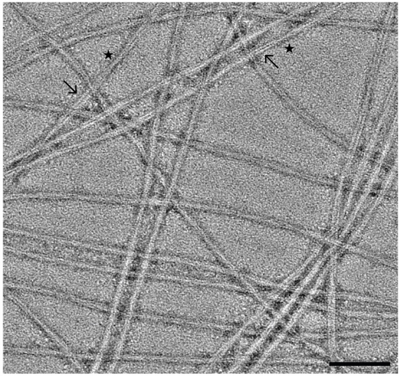
Representative micrograph of fibrils lightly stained with 1% UA. The in vitro fibrils are comprised of two protofilaments (arrows) and appear to be twisting with distinct crossover points (stars). These fibrils are long enough to span the micrograph, demonstrate an optimized preparation, are not overcrowded indicating appropriate concentration, and have minimal overlap to allow for adequate particle picking. Additionally, the micrograph did not appear to contain aggregates, contaminates, or extra biological material. This is optimal for data collection/processing and represents an encouraging negative stain screen. Scale bar, 100 nm.
1. Place the desired number of 200 mesh carbon film, copper EM grids on a grid holder block and use a plasma cleaner (PDC-32G or equivalent system) to glow discharge grids under a 100-micron vacuum for 30 s on low (Figure 3, step 1).
2. Cut a piece of parafilm to approximately 2” × 4” and demagnetize with a static dissipater (Figure 3, step 2).
3. Retrieve one glow-discharged EM grid using style N5 reverse pressure tweezers or similar tweezers (Figure 3, step 3).
4. Spot two 50 μL drops of sterile, Nanopure water and two 50 μL drops of 1% UA onto the piece of parafilm. Ensure the drops do not touch (Figure 3, step 4).
5. Apply 4 μL of the sample to the EM grid and allow the sample to incubate at room temperature for 1 min (Figure 3, step 5).
6. Blot away the liquid by touching the edge of the EM grid to a piece of filter paper (Figure 3, step 6).
7. Wash the EM grid by touching the face of the EM grid to the first drop of water and then blot away the liquid as in step B6. Repeat, but this time wash with the second drop of water (Figure 3, step 7).
8. Pre-stain the EM grid by touching the face of the EM grid to the first drop of 1% UA, then blot away the stain as in step B6 (Figure 3, step 8).
9. Stain the grid by holding the face of the EM grid to the second drop of 1% UA for 15 s, then blot away the stain as in step B6 (Figure 3, step 9).
10. Allow the EM grid to dry for at least 5 min at room temperature before storing the grid in a grid box (Figure 3, step 10). Store the grid box in a desiccator or humidity-controlled room until imaging.
11. Repeat for additional sample dilutions to assess the sample conditions that may be best suited for cryo-EM analysis. We imaged the sample at a concentration of 13 mg/mL (undiluted), 6.5 mg/mL (2× dilution), and 2.6 mg/mL (5× dilution). We found that a concentration of 6.5 mg/mL showed the best sample distribution on the grid (Figure 4).
Note: Since fibrilization conditions greatly impact the length of the fibrils and thus the sample distribution on the grid, it is important to test each sample by NS-TEM before sample vitrification and cryo-EM data collection.
12. Image grids on a Talos L120C 120 kV TEM or equivalent microscope at a pixel size of 1.58 Å and a total electron dose of ~25 e-/Å2.
C. Sample vitrification
Basic sample vitrification for single particle analysis has become routine in the cryo-EM field. Here, we present a brief workflow of the vitrification process using the Vitrobot Mark IV with blotting conditions that yield grids suitable for cryo-EM data collection.
1. Using a plastic syringe, add 60 mL of distilled water to the Vitrobot Mark IV water reservoir.
2. Turn on the Vitrobot Mark IV and set the chamber temperature to 20 °C and the relative humidity to 95%.
3. Attach standard Vitrobot filter paper to the blotting pads and allow the system to equilibrate to the conditions set in step C2 (~15 min).
4. Using a plasma cleaner or equivalent system, glow-discharge R2/1 200 mesh, copper grids.
5. Use liquid nitrogen (LN2) to cool the Vitrobot foam dewar, ethane cup, and metal spider.
6. Once the setup has cooled, condense the ethane in the ethane cup. Be sure to monitor ethane and LN2 levels throughout the vitrification process.
7. On the Vitrobot, set the wait time to 60 s and set the drain time to 0.5 s. For blot force and blot time, it is usually necessary to test a range of parameters that work best. For these fibrils, a blot time between 4 and 5 s and a blot force of -1 to +2 worked well.
Note: There is variance between Vitrobots; thus, optimization of blotting force and blot time may be necessary for the specific equipment being used.
8. Using the Vitrobot tweezers, pick up a grid and attach the tweezers to the Vitrobot. Select continue on the screen to raise the tweezers and mount the foam dewar in place. Follow the prompts on the screen to bring the tweezers and dewar into position for sample application.
9. Apply 4 mL of the fibrils to the carbon side of the grid. Select continue to begin the wait time; then, the system will automatically blot and plunge the sample into liquid ethane.
10. Once the system has plunged the specimen into the cryogen, transfer the vitrified grid to a labeled grid box and store appropriately.
Note: A complete guide on plunge freezing using the Vitrobot can be found in unit 2 of the Getting Started with Cryo-EM videos ( https://youtube.com/playlist?list=PL8_xPU5epJdfd5fM2CjQItR-iRlIEIJk8&si=NAqencnr2wpuZg9B ).
11. Repeat steps C7–9 for any additional grids. In addition to duplicate grids, it is always beneficial to test a range of blotting conditions and/or sample concentrations. Cryo-EM data was collected on a grid with a blot time of 4 s and a blot force of +2 at a protein concentration of ~6.5 mg/mL.
D. Cryo-EM data collection
Data collection parameters should be tailored to the resources available, and thus users should work closely with EM facility staff to optimize the data collection parameters for their individual sample. Here, the data was acquired on a Titan Krios G3i FEG-TEM. The microscope is operated at 300 kV and is equipped with a Gatan K3 direct electron detector and a BioQuantum energy filter set at 20 eV. Correlated double sampling (CDS) was used to collect dose-fractionated micrographs using a defocus range of -0.5 to -2.5 μm with increments of 0.25 μm. Micrographs were collected at a magnification of 105,000× with a pixel size of 0.834 Å and a total dose of 40 e-/Å2 (1 e-/Å2/frame). On average, ~250 movies were collected per hour using EPU/AFIS (Thermo Fisher Scientific) acquiring three shots per hole and multiple holes per stage movement. A representative micrograph at an estimated defocus of -2.0 μm shows twisting fibrils suspended in vitreous ice (Figure 5).
Figure 5. Representative cryo-EM micrographs of a-synuclein fibrils.
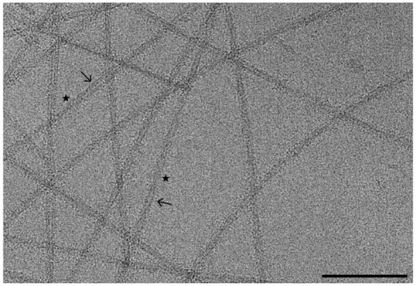
Motion-corrected micrograph of vitrified a-syn fibrils at an estimated defocus of -2.0 μm. The fibrils are comprised of two protofilaments (arrows) that are twisting at distinct crossover points (stars). Twisting fibrils are critical for high-resolution structure determination. Scale bar, 100 nm.
E. Cryo-EM data processing of a-synuclein fibrils
Cryo-EM structure determination of amyloid fibrils has revolutionized the fields of neuroscience and neurodegenerative medicine, providing key structural details that were previously unattainable by other methods. Here, we provide a data processing protocol that is both detailed and reproducible to serve as a starting point for those new to cryo-EM and helical reconstruction workflows. The raw micrographs, gain file, and the detector mtf file can be accessed at EMPIAR-12229, allowing users to work through the steps below before applying the workflow to new experimental data. We must note that all data sets are unique and possess their own challenges, but this workflow should greatly improve the user’s ability to resolve amyloid fibril structures. Finally, as with any software, it is best to first become accustomed to the program by completing the appropriate tutorial datasets. We highly encourage readers to first complete the RELION single particle tutorial (https://relion.readthedocs.io/en/release-4.0/SPA_tutorial/index.html) before proceeding with the steps below [36].
Creating a RELION Project
Create a directory that will house the entire RELION project. For simplicity, call this directory a-syn_data_processing. Within this directory, you should have two files titled gain.mrc and k3-CDS-300keV-mtf.star and a subdirectory titled Micrographs that contains all the raw movie frames in tiff format. These files can be downloaded from EMPIAR-12229. Now that your directories are organized, cd to the a-syn_data_processing directory, this will serve as the RELION parent directory for all subsequent jobs. Launch RELION by running relion & in the terminal. The “&” will allow RELION to run in the background in case the terminal is needed for additional commands. As a final note, we have listed the input files for each job based on our RELION project so there will be discrepancies in job numbers between our project and yours. Thus, it is important to use the proper input path file for your project at each step. For each step, we have detailed where the input file comes from (i.e., the step the file was generated in) to ensure successful reconstruction of the EMPIAR-12229 dataset.
Allocating computational resources when running RELION jobs
RELION uses a Compute and Running tab to allocate computational resources based on user-defined parameters. These parameters are completely dependent on the resources available to each individual. Thus, rather than detailing these parameters for each step, here we have outlined the Compute and Running parameters that work well for our HPC cluster with slurm queueing system. However, these parameters may not work for your computational setup, and you may need to seek the advice of IT professionals at your institute. We have also included the Compute and Running tabs in Video 1 for each job as an additional resource for determining these parameters.
Video 1. RELION-4 parameters for the helical reconstruction of a-synuclein fibrils.
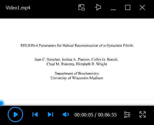
Screenshots of the RELION GUI for each step from section E are provided for easier visualization of input parameters. Additional information regarding the origin of the input files is provided, as the file names will vary from project to project depending on the number of RELION jobs run.
Compute
Use parallel disk I/O? Yes
Number of pooled particles: 30
Skip padding? No
Pre-read all particles into RAM? No
Copy particles to scratch directory: Leave Blank
Combine iterations through disc? No
Use GPU acceleration? Yes
Which GPUs to use: Leave Blank
Running (GPU jobs):
Number of MPI procs: 5
Number of threads: 6
Submit to queue? Yes
Queue name: a5000
Queue submit command: sbatch
Standard submission script: ../../../../../../share/sbatch/relion_template_gpu.sh
Minimum dedicated cores per node: 1
Additional arguments: Leave Blank
Running (CPU jobs):
Number of MPI procs: 20
Submit to queue? Yes
Queue name: cpu
Queue submit command: sbatch
Standard submission script: ../../../../../../share/sbatch/relion_template_cpu.sh
Minimum dedicated cores per node: 1
Additional arguments: Leave Blank
In addition to the protocol below, a workflow diagram and a video of the RELION GUI with parameters for each step are provided (Figure 6, Video 1).
Figure 6. Helical reconstruction workflow for a-synuclein fibrils using RELION.

Overview of each RELION job utilized to reconstruct a-syn fibrils to ~2.0 Å. Each job corresponds to the step number in section E and to those in Video 1.
1. Import
First, import the raw movie frames into RELION for data processing. Select the Import job, ensure Raw input files is set to the location of the movie frames, use the “*” argument to select all the tiff files in the directory, set the additional parameters below, and click the Run! button.
Movies/mics:
Import raw movies/micrographs: Yes
Raw input files: Micrographs/*.tiff
Optics group name: opticsGroup1
MTF of the detector: k3-CDS-300keV-mtf.star
Pixel size (Angstrom): 0.834
Voltage (kV): 300
Spherical aberration (mm): 2.7
Amplitude contrast: 0.1
Beamtilt in X (mrad): 0
Beamtilt in Y (mrad): 0
Others:
Import other node types? No
The output log will display 5,193 micrographs imported.
2. Motion correction
The raw movie frames from the previous job (movies.star) must now be aligned. The data was collected with a dose per frame of 1 e-/Å2 over 40 frames for a total dose of 40 e-/Å2. Note that the EER fractionation parameter will be ignored by RELION since these images were collected on a Gatan K3 detector and are tiff files. Perform motion correction by using the MotionCor2 program [38]. Tell RELION where the program is located via the MOTIONCOR2 executable parameter. Your computational setup will be different, and MotionCor2 may be saved in a different location, so the executable path may be different. In the terminal, run which motioncor2 to determine the correct path for the program. Similarly, your computational setup will dictate the number of GPUs available. Our setup includes multiple nodes, and each can run 4 GPUs concurrently. In the RELION GUI, use Which GPUs to use to indicate the GPUs available for your setup; leaving this blank will automatically allocate the GPUs. Select the Motion correction job, set Input movies STAR file to the movie.star file from step 1, set the following parameters and update any paths or parameters that are specific to your computational setup, and then click the Run! button.
I/O:
Input movies STAR file: Import/job001/movies.star
First frame for corrected sum: 1
Last frame for corrected sum: -1
Dose per frame (e-/Å2): 1
Pre-exposure (e-/Å2): 0
EER fractionation: 32
Write output in float16? Yes
Do dose-weighting? Yes
Save non-dose weighted as well? No
Save sum of power spectra? Yes
Sum power spectra every (e-/Å2): 4
Motion:
Bfactor: 150
Number of patches X, Y: 5, 5
Group frames: 1
Binning factor: 1
Gain-reference image: gain.mrc
Gain rotation: 180 degrees (2)
Gain flip: Flip left to right (2)
Defect file: Leave blank
Use RELION’s own implementation? No
MOTIONCOR2 executable: /programs/x86_64-linux/motioncor2/1.3.1/motioncor2
Which GPUs to use: 0,1,2,3
Other MOTIONCOR2 arguments: Leave blank
This job will take several hours to run and will generate a corrected_micrographs.star file. If interested, you may open the logfile.pdf to visualize the results from the job. Under the Finished Jobs list click on the Motion correction job. This will update the Current: job display (located in the center of the GUI) to your Motion correction job and upload the results to the user interface. On the right side of the RELION GUI there is a drop-down menu called Display: that allows the user to visualize outputs from the finished job. Click on the drop-down menu and select Out: logfile.pdf. A new window will appear with the results of the job. Subsequent logfile.pdf files from finished jobs can be opened this way.
3. CTF estimation
Now, estimate the CTF values for the motion-corrected micrographs from the previous step; these are stored in the corrected_micrographs.star file. Use Gctf to estimate CTF values [39]. In the terminal, run which Gctf to determine the correct executable path for your setup. In the RELION GUI, select the CTF estimation job, set Input micrographs STAR file to the corrected_micrographs.star file from step 2, set the following parameters and update any paths specific to your setup, and then click the Run! button.
I/O:
Input micrographs STAR file: MotionCorr/job002/corrected_micrographs.star
Use micrograph without dose-weighting? No
Estimate phase shifts? No
Amount of astigmatism (Å): 100
CTFFIND-4.1:
Use CTFFIND-4.1? No
FFT box size (pix): 512
Minimum resolution (Å): 30
Maximum resolution (Å): 5
Minimum defocus value (Å): 5000
Maximum defocus value (Å): 50000
Defocus step size (Å): 500
Gctf:
Use Gctf instead? Yes
Gctf executable: /programs/x86_64-linux/gctf/1.06/bin/Gctf
Ignore ‘Searches’ parameters? Yes
Perform equi-phase averaging? Yes
Other Gctf options: Leave blank
Which GPUs to use: 0,1,2,3
This job results in a micrographs_ctf.star file and a logfile.pdf file. The logfile.pdf contains a graphical representation of the metadata related to micrograph defocus, astigmatism, max resolution, and figure of merit values. These values will be used in the upcoming steps to filter the micrograph dataset.
4. Subset selection (defocus filter)
Extensive testing has shown that using stringent parameters during the micrograph curation steps allows for a segment picking neural network that performs better than one trained on the entire data set. The following steps will use CTF estimation results to curate a set of micrographs for manual picking. Those picks will then be used to train the Topaz neural network [40]. Finally, a modified version of Topaz called Topaz-filament, which allows for picking filamentous structures, is optimized on a small subset of micrographs before applying the neural network to our entire dataset [40].
Open the logfile.pdf from the CTF estimation job and use the values provided in this file to eliminate any outliers or suboptimal micrographs. Filter the dataset based on defocus, astigmatism, max resolution, and figure of merit values using a series of Subset Selection jobs. Select the Subset Selection job, input the following parameters and update OR select from micrograph.star to the micrographs_ctf.star file from step 3, and then click the Run! button.
I/O:
Select classes from job: Leave blank
OR select from micrograph.star: CtfFind/job003/micrographs_ctf.star
OR select from particles.star: Leave blank
Class options:
Automatically select 2D classes? No
Re-center the class averages? No
Regroup the particles? No
Subsets:
Select based on metadata value? Yes
Metadata label for subset selection: rlnDefocusU
Minimum metadata value: -9999
Maximum metadata value: 25000
OR: select on image statistics? No
OR: split into subsets? No
Duplicates:
OR: remove duplicates? No
This job reduces the number of micrographs from 5,193 to 4,858 based on a maximum defocus value of 2.5 mm (25,000 Å).
5. Subset selection (astigmatism filter)
Filter the micrograph subset from step 4 by the astigmatism values in the CTF estimation logfile.pdf file. Select the Subset Selection job type, set OR select from micrograph.star to the micrographs.star file from step 4, input the following parameters, and then click the Run! button.
I/O:
Select classes from job: Leave blank
OR select from micrograph.star: Select/job004/micrographs.star
OR select from particles.star: Leave blank
Class options:
Automatically select 2D classes? No
Re-center the class averages? No
Regroup the particles? No
Subsets:
Select based on metadata value? Yes
Metadata label for subset selection: rlnCtfAstigmatism
Minimum metadata value: -9999
Maximum metadata value: 700
OR: select on image statistics? No
OR: split into subsets? No
Duplicates:
OR: remove duplicates? No
This job reduces the number of micrographs from 4,858 to 3,390 micrographs.
6. Subset selection (max resolution filter)
Further filter the micrograph subset from step 5 by the max resolution values from the CTF estimation logfile.pdf file. Select the Subset Selection job, set OR select from micrograph.star to the micrograph.star file from step 5, set the following parameters, and click the Run! button.
I/O:
Select classes from job: Leave blank
OR select from micrograph.star: Select/job020/micrographs.star
OR select from particles.star: Leave blank
Class options:
Automatically select 2D classes? No
Re-center the class averages? No
Regroup the particles? No
Subsets:
Select based on metadata value? Yes
Metadata label for subset selection: rlnCtfMaxResolution
Minimum metadata value: -9999
Maximum metadata value: 4
OR: select on image statistics? No
OR: split into subsets? No
Duplicates:
OR: remove duplicates? No
This job reduces the number of micrographs from 3,390 to 910 micrographs.
7. Subset selection (figure of merit filter)
Lastly, filter the micrograph subset from step 6 by the figure of merit values from the CTF estimation logfile.pdf file. Select the Subset Selection job, set OR select from micrograph.star to the micrograph.star file from step 6, set the following parameters, and then click the Run! button.
I/O:
Select classes from job: Leave blank
OR select from micrograph.star: Select/job021/micrographs.star
OR select from particles.star: Leave blank
Class options:
Automatically select 2D classes? No
Re-center the class averages? No
Regroup the particles? No
Subsets:
Select based on metadata value? Yes
Metadata label for subset selection: rlnCtfFigureOfMerit
Minimum metadata value: 0.065
Maximum metadata value: 0.9
OR: select on image statistics? No
OR: split into subsets? No
Duplicates:
OR: remove duplicates? No
This job reduces the number of micrographs from 910 to 774 micrographs.
8. Subset selection (2 sets of 20 micrograph)
From the remaining 774 micrographs, generate 2 sets of 20 micrographs. The first set of micrographs will be used for manual picking and training the neural network. The second set of 20 micrographs will be used to test and optimize the picking thresholds that will then be applied to the entire dataset. Select the Subset Selection job, set OR select from micrograph.star to the micrographs.star file from step 7, and then click the Run! button.
I/O:
Select classes from job: Leave blank
OR select from micrograph.star: Select/job022/micrographs.star
OR select from particles.star: Leave blank
Class options:
Automatically select 2D classes? No
Re-center the class averages? No
Regroup the particles? No
Subsets:
Select based on metadata value? No
OR: select on image statistics? No
OR: split into subsets? Yes
Randomise order before making subset? No
Subset size: 20
OR: number of subsets: 2
Duplicates:
OR: remove duplicates? No
This step results in two STAR files labeled micrographs_split1.star and micrographs_split2.star. Each star file contains 20 micrographs.
9. Manual picking
Select the Manual picking job, set Input micrographs to the micrographs_split1.star file from step 8, set the additional parameters below, and then click the Run! button. A new window will appear with 20 rows (one per micrograph) with the micrograph name, a pick button, the number of picks, a CTF button, and the defocus estimate for that micrograph. Click on the pick button to launch a new window for the specified micrograph. Use the left mouse button and click at one end of a fibril, and then click a second time at the opposite end of the fibril. This creates a line segment between the two endpoints defined by the user. The segments will be used for the particle extraction job in subsequent steps. Repeat this process until all the fibrils are picked. Ensure segments do not overlap; if fibrils contain curvature, increase the number of segments that make up the filament (Figure 7A). When done picking, right-click on the micrograph and select Save STAR with coordinates, close the micrograph, and repeat the process for the remaining 19 micrographs. If you need to remove points, use the center button and click over an existing point to remove it. Ensure that all the micrographs have an even number of picks (i.e., one start point and one end point per segment) and that segments are centered over fibrils. When done picking from all 20 micrographs, close the window to finalize the job.
Figure 7. Manual picking, 2D class selection, and auto-picking threshold determination.

A. Micrograph with examples of manually picked segments (step 9). Each “end” of the segment is selected by the user (indicated by the stars). The endpoints are then linked by a line (indicated by an arrow); this region will be divided into particles based on the user-defined interbox distance. Each new color represents a new segment that has been manually picked. B. Schematic of interbox distances (step 10). The filament that is shown is a region that has been selected for particle picking. RELION will use a user-defined “box” to select as a particle. The interbox distance shown is the distance in which no overlap from previous boxes is present (i.e., the region that is unique to each box). C. 2D classes from manually picked particles (step 11). The green boxes indicate the classes selected to use for neural network training (step 12). D. Micrographs depicting trained neural network auto-picking results from different threshold values. As the threshold for picking is decreased, the stringency in which the neural network determines whether the feature fits the trained model is decreased, initially resulting in an increase in picked particles. However, as the threshold continues to decrease, the neural network starts to categorize “noise” as pickable particles.
I/O:
Input micrographs: Select/job023/micrographs_split1.star
Pick start-end coordinates helices? Yes
Use autopick FOM threshold? No
Display:
Particle diameter (Å): 100
Scale for micrographs: 0.2
Sigma contrast: 3
White value: 0
Black value: 0
Lowpass filter (Å): 20
Highpass filter (Å): -1
Pixel size (Å): -1
OR: use Topaz denoising? No
Colors:
Blue<>red color particles? No
The output log will list the total number of picks (start and end points). Here, we picked 414 particles (i.e., 207 segments) from 20 micrographs, and the coordinates are saved to the manualpick.star file located in the directory for this job. The total number of segments may vary due to differences in picking, but ensure picks are made on all 20 micrographs.
Note: The parameters in the Display tab are for visualization purposes only and do not impact downstream processing steps.
Note: We observed that in some versions of RELION there is a bug that results in an empty coordinate file from the Manual picking job. To bypass this error, simply select the Manual picking job from the Finished jobs section and then click on the Continue! button. This will reopen the manual picking GUI. Then, close the window; the coordinate file should now be updated with all the picks saved. There is no need to repick particles or change any settings.
10. Particle extraction (manual picks)
The manually picked segments must now be processed to extract particles for 2D classification. In principle, this step will take user-defined parameters to then cut the segments into individual particles for downstream steps (Figure 7B). This is achieved by providing the number of unique asymmetrical units and helical rise (Å) values in the helix tab. RELION will use these values to establish an interbox distance, i.e., the spacing between each particle, that will separate overlapping 360-pixel boxes that traverse the length of the segment (Figure 7B). Here, we have set the interbox distance to ~38.5 Å (4.82 Å × 8) to increase the number of particles for training purposes. This value will be expanded later once auto-picking is complete. Select the Particle extraction job, set Micrograph STAR file to the micrograph_split1.star file from step 8, set Input coordinates to the manualpick.star file from step 9, and then click the Run! button.
I/O:
Micrograph STAR file: Select/job023/micrographs_split1.star
Input coordinates: ManualPick/job024/manualpick.star
OR re-extract refined particles? No
OR re-center refined coordinates? No
Write output in float16? Yes
Extract:
Particle box size (pix): 360
Invert contrast? Yes
Normalize particles? Yes
Diameter background circle (pix): -1
Stddev for white dust removal: -1
Stddev for black dust removal: -1
Rescale particles? No
Use autopick FOM threshold? No
Helix:
Extract helical segments? Yes
Tube diameter (Å): 140
Use bimodal angular priors? Yes
Coordinates are start-end only? Yes
Cut helical tubes into segments? Yes
Number of unique asymmetrical units: 8
Helical rise (Å): 4.82
This job resulted in 5,919 particles extracted to a pixel size of 0.834 Å/pix with a box size of 360 pixels. Differences in particle counts are due to differences in the number of segments picked during the manual picking step. Aim for at least 4,000 particles at this stage.
Note: Amyloid structures have a consistent helical rise of ~4.8 Å. This estimate is sufficient for this stage of processing, as the helical rise will be optimized in subsequent steps.
11. 2D classification (manual picks)
Although the particles were manually picked and thus should be free from suboptimal picks or background noise, we prefer to perform a round of 2D classification to curate the particles that will be used to train the Topaz neural network. Select the 2D classification job, set Input images STAR file to the particles.star file from step 10, set the parameters below, and then click on the Run! button.
I/O:
Input images STAR file: Extract/job029/particles.star
CTF:
Do CTF-correction? Yes
Ignore CTFs until first peak? No
Optimisation:
Number of classes: 20
Regularisation parameter T: 2
Use EM algorithm? Yes
Number of EM iterations: 20
Use VDAM algorithm? No
Mask diameter (Å): 285
Mask individual particles with zeros? Yes
Limit resolution E-step to (Å): 10
Center class averages? Yes
Sampling:
Perform image alignment? Yes
In-plane angular sampling: 2
Offset search range (pix): 5
Offset search step (pix): 1
Allow coarser sampling? No
Helix:
Classify 2D helical segments? Yes
Tube diameter (Å): 140
Do bimodal angular searches? Yes
Angular search range-psi (deg): 6
Restrict helical offsets to rise: Yes
Helical rise (Å): 4.82
Due to the small number of particles and the small number of classes, this job should only take a couple of minutes to run. The final classes can be visualized by clicking on the Display: drop-down menu and selecting out: run_it020_optimiser.star. A RELION display GUI will appear; check the box next to Sort images on: and select rlnClassDistribution from the drop-down menu, then click Display! to see the classes sorted with the most populated classes at the top (Figure 7C). Close the window when done.
12. Subset selection (2D classes for Topaz training)
Next, use the Subset selection job to select the best classes to train the Topaz neural network. Set Select classes from job to the run_it020_optimiser.star file from step 11, set the additional parameters below, and click the Run! button. This will launch a RELION display GUI. Check the box next to Sort images on: and select rlnClassDisribution, then click the Display! button. This will look identical to the previous step where we visualized the classes, but now you use the left mouse button to select all the classes to move to the next step (Figure 7C). Once done, right-click and select Save selected classes, then close the display window.
I/O:
Select classes from job: Class2D/job030/run_it020_optimiser.star
OR select from micrograph.star: Leave blank
OR select from particles.star: Leave blank
Class options:
Automatically select 2D classes? No
Re-center the class averages? Yes
Regroup the particles? No
Subsets:
Select based on metadata values? No
OR: select on image statistics? No
OR: split into subsets? No
Duplicates:
OR: remove duplicates? No
This job resulted in 15 classes selected with 5,712 particles (Figure 7C, green boxes). Your values may be slightly different at this step due to differences in manual picking, but the key is to select classes that appear fibrillar in nature (Figure 7C, green boxes).
13. Auto-picking (Topaz training)
Use the curated particle stack to train a new Topaz neural network. It is critical that the executable path within the Topaz tab directs RELION to the topaz-filament program [40]. The path here is to where topaz-filament is located on our HPC cluster, but this may be different for your setup. If you are unsure where this program is located, you may attempt to locate the program path by running the which topaz-filament command from the terminal. Select the Auto-picking job, set Input micrographs for autopick to the micrographs_selected.star file from step 9, in the Topaz tab set Particles STAR file for training to the particles.star file from step 12, set the additional parameters below and modify the executable path to fit your computational setup, and then click on the Run! button.
I/O:
Input micrographs for autopick: ManualPick/job024/micrographs_selected.star
Pixel size in micrographs (Å): -1
Use reference-based template-matching? No
OR: use Laplacian-of-Gaussian? No
OR: use Topaz? Yes
Laplacian:
This tab is ignored since we opted to use Topaz in the I/O tab.
Topaz:
Topaz executable: /programs/x86_64-linux/system/sbgrid_bin/topaz-filament
Particle diameter (Å): 140
Perform topaz picking? No
Perform topaz training? Yes
Nr of particle per micrograph: 300
Input picked coordinates for training: Leave blank
OR train on a set of particles? Yes
Particles STAR file for training: Select/job032/particles.star
Additional topaz arguments: Leave blank
References:
This tab is ignored since we opted to use Topaz in the I/O tab.
Autopicking:
Use GPU acceleration? Yes
All other parameters on this tab are ignored since we opted to use Topaz in the I/O tab.
Helix:
This tab is ignored since we opted to use Topaz in the I/O tab.
This job results in a trained Topaz model titled model_epoch10.sav which is saved in the folder for this job.
Note: Topaz training is not parallelized, so the job will only use one MPI process.
14. Auto-picking (Topaz picking optimization)
The trained Topaz model will be applied to a subset of 20 micrographs to test how the model performs before it is applied to the entire dataset. For topaz-filament to pick segments and not individual particles as in traditional single particle analysis, the additional flags for filament (-f) and threshold (-t) must be provided in the Additional topaz arguments box. Additionally, an integer value must be provided after the threshold flag. This threshold determines how many particles are picked. A lower threshold results in more particles, but if the threshold is too low, then the model will start picking noise. With any new trained Topaz neural network, we test a range of threshold values, typically from -6 to 0, to see which threshold works best (Figure 7D). Each threshold value will be its own job. Select the Auto-picking job, set Input micrographs for autopick to the micrographs_split2 from job 8, in the Topaz tab set Trained topaz model to the model_epoch10.sav file from step 13, set the parameters below, and click the Run! button. To test additional thresholds, once the first Auto-picking job is complete, click on the job in the Finished jobs list and then click on the Auto-picking job to load the previous settings. Now, simply change the threshold value in the Additional topaz arguments and click the Run! button. Repeat this process for any threshold that you would like to test. We tested thresholds -6, -5, -4, -3, -2, -1, and 0, and found that threshold -5 worked best for the dataset (Figure 7D). We have also included an extreme case with a threshold of -10 to better visualize bad picks that would be unsuitable for further processing (Figure 7D).
I/O:
Input micrographs for autopick: Select/job023/micrographs_split2.star
Pixel size in micrographs (Å): -1
Use reference-based template-matching? No
OR: use Laplacian-of-Gaussian? No
OR: use Topaz? Yes
Laplacian:
This tab is ignored since we opted to use Topaz in the I/O tab.
Topaz:
Topaz executable: /programs/x86_64-linux/system/sbgrid_bin/topaz-filament
Particle diameter (Å): 140
Perform topaz picking? Yes
Trained topaz model: AutoPick/job033/model_epoch10.sav
Perform topaz training? No
Additional topaz arguments: -f -t -5
References:
This tab is ignored since we opted to use Topaz in the I/O tab.
Autopicking:
Use GPU acceleration? Yes
All other parameters on this tab are ignored since we opted to use Topaz in the I/O tab.
Helix:
This tab is ignored since we opted to use Topaz in the I/O tab.
A picking threshold of -5 resulted in 688 segments (1,376 particles, i.e., endpoints) from 20 micrographs.
Note: Topaz picking is parallelized so multiple MPI processes can be run simultaneously; we typically run 20 MPI processes for this job. This setting can be found in the Running tab and is dependent on the computational resources available.
15. Auto-picking (Topaz picking on the entire dataset)
The trained Topaz model and the optimized picking threshold are now applied to the entire dataset to select segments for downstream processing. As detailed previously, upload the settings from the best picking job (threshold -5), update Input micrographs for autopick to the micrographs.star file from step 4, and click the Run! button.
I/O:
Input micrographs for autopick: Select/job004/micrographs.star
Pixel size in micrographs (Å): -1
Use reference-based template-matching? No
OR: use Laplacian-of-Gaussian? No
OR: use Topaz? Yes
Laplacian:
This tab is ignored since we opted to use Topaz in the I/O tab.
Topaz:
Topaz executable: /programs/x86_64-linux/system/sbgrid_bin/topaz-filament
Particle diameter (Å): 140
Perform topaz picking? Yes
Trained topaz model: AutoPick/job033/model_epoch10.sav
Perform topaz training? No
Additional topaz arguments: -f -t -5
References:
This tab is ignored since we opted to use Topaz in the I/O tab.
Autopicking:
Use GPU acceleration? Yes
All other parameters on this tab are ignored since we opted to use Topaz in the I/O tab.
Helix:
This tab is ignored since we opted to use Topaz in the I/O tab.
This job results in 156,526 segments (313,052 particles, i.e., endpoints) from 4,858 micrographs.
16. Particle extraction (large box size)
For helical reconstruction methods, the helical twist and rise values are critical for cryo-EM data processing. The helical twist can be estimated from 2D class averages with large box sizes that span the fibril crossover distance (Figure 8A, 8B, 8D). Here, extract the particles to a box size of 864 pixels (~720 Å) so we can estimate the crossover distance in subsequent steps. At this stage in the processing, there is no need for high-resolution information, so the box size is rescaled to 144 pixels (i.e., binning to a pixel size of 5.004 Å/pixel). Alternatively, users may estimate the crossover distance from cryo-EM micrographs (typically those with higher defocus values are easier to visualize) or from negative stain TEM micrographs. However, extraction at a larger box size is still necessary to generate an initial reference for 3D reconstruction. Select the Particle extraction job, set Micrograph STAR file to the micrographs.star file from step 4, set Input coordinates to the autopick.star file from step 15, set the additional parameters below, and click the Run! button.
Figure 8. Determining crossover distance, helical twist, and helical rise.

A. An initial map depicts the crossover distance observed in twisting fibrils. The crossover distance is described as the length where the fibril turns 180° (red dotted line). Scale bar, 100 nm. B. The crossover distance can be measured (red line) from well-aligned 2D classes where the twisting nature of the fibril is observed; this requires a box size that spans a distance that is close to or larger than the crossover distance for an accurate measurement to be made. Here, a box size of 864 pixels (720 Å) was used for initial crossover estimates. Poor 2D classes that are misaligned or blurry prevent crossover distance measurements. C. The helical rise can be determined from 2D classes with a small box size (360 pixels) extracted at their original pixel size (0.834 Å/pix) that yield high-resolution details (i.e., spacing of the β-sheets). The sigma contrast of the 2D classes must be adjusted to visualize the helical layer lines in reciprocal space. From the average power spectrum, a measurement (red line) can be made from the meridian to the highest intensity layer line. This measurement can be used to estimate the helical rise. D. The measurements made in B and C are used to calculate the helical rise and the crossover distance. Then, the crossover distance and helical rise are used to calculate the helical twist of the structure. The estimated helical parameters are used for subsequent 3D refinement steps.
I/O:
Micrograph STAR file: Select/job004/micrographs.star
Input coordinates: AutoPick/job041/autopick.star
OR re-extract refined particles? No
OR re-center refined coordinates? No
Write output in float16? Yes
Extract:
Particle box size (pix): 864
Invert contrast? Yes
Normalize particles? Yes
Diameter background circle (pix): -1
Stddev for white dust removal: -1
Stddev for black dust removal: -1
Rescale particles? Yes
Re-scale size (pixels): 144
Use autopick FOM threshold? No
Helix:
Extract helical segments? Yes
Tube diameter (Å): 140
Use bimodal angular priors? Yes
Coordinates are start-end only? Yes
Cut helical tubes into segments? Yes
Number of unique asymmetrical units: 15
Helical rise (Å): 4.82
This job results in 771,754 particles with an original box size of 864 pixels that is rescaled to 144 pixels at a pixel size of 5.004 Å/pixel.
Note: The number of asymmetrical units was increased to 15. This results in an interbox distance of ~72 Å or ~25% of the small box size (360 pixels) that will be used for the final reconstruction.
17. 2D classification (large box size)
Classify the particles to remove junk particles and to estimate the crossover distance. Select the 2D classification job, set Input images STAR file to the particles.star file from step 16, set the additional parameters below, and then click on the Run! button.
I/O:
Input images STAR file: Extract/job042/particles.star
CTF:
Do CTF-correction? Yes
Ignore CTFs until first peak? Yes
Optimisation:
Number of classes: 50
Regularisation parameter T: 2
Use EM algorithm? Yes
Number of EM iterations: 20
Use VDAM algorithm? No
Mask diameter (Å): 710
Mask individual particles with zeros? Yes
Limit resolution E-step to (Å): -1
Center class averages? Yes
Sampling:
Perform image alignment? Yes
In-plane angular sampling: 2
Offset search range (pix): 5
Offset search step (pix): 1
Allow coarser sampling? No
Helix:
Classify 2D helical segments? Yes
Tube diameter (Å): 140
Do bimodal angular searches? Yes
Angular search range-psi (deg): 6
Restrict helical offsets to rise: Yes
Helical rise (Å): 4.82
This job results in the run_it020_optimiser.star file that contains the 2D class averages. This file can be viewed using the Display: drop-down menu on the right side of the GUI.
Sometimes, it can be helpful to determine the helical rise of the filament rather than assume 4.8 Å as the starting point. To do this, users can utilize 2D classifications and measurements of the average power spectra in Fourier space to calculate the estimated rise. To perform this analysis, use a box size of 360 pixels and high-resolution data (0.834 Å/pix), as this allows for more detail to be visualized in the 2D classes (specifically the β-sheet rungs). To do so, use the Particle Extraction job to extract particles to their original pixel size. Use the parameters as instructed in step 16, but ensure that Particle box size is set to 360 and that Rescale particles is set to No. Once particle extraction is complete, run a 2D Classification job as described in step 17. Ensure Input images STAR files is set to the correct particles.star file from the Particle Extraction job and Mask diameter is set to 300. When the job is done, open the average power spectra by selecting the out:run_it020_optimiser from the display output. Enter an increased Sigma Contrast value in the top box of the RELION display GIU (we used 1 for our data) (Figure 8C). If the user fails to increase the Sigma Contrast, the average power spectra will not be visible (Figure 8C). Once the 2D classes are displayed, right-click on a class and select Show Fourier amplitudes (2X). This will open an image of the average power spectra. Make a measurement from the meridian to either layer line with the strong intensity (Figure 8C). This can be done by clicking and holding the center button on the mouse. Use the following formula to calculate the rise: (Figure 8C, 8D). For new experimental data, if the rise is substantially different, then parameters for steps 16 onward should reflect the updated rise. Here, a measurement of ~124 pixels results in a helical rise of 4.84 Å that will be refined in later steps (Figure 8C).
18. Subset selection (2D classes for initial map)
Select 2–3 good classes that will be used to generate an initial 3D volume. Select the Subset Select job, set Select classes from job to the run_it020_optimiser.star file from step 17, set the parameters below, then click the Run! button. A RELION display GUI will appear; reverse sort the class averages by rlnClassDistribution (as described in step 11) and select 2 class averages (Figure 9A, green boxes). To measure the crossover distance, right-click on a 2D class and select Show original image. A new window will appear. Using the center button, click and drag to measure the distance between two crossovers (Figure 8B). The distance in pixels is displayed over the image and in the terminal (Figure 8B). Multiply the measured distance by the current pixel size of 5.004 Å/pixel to calculate the distance in angstroms (Figure 8D). Here, we estimated a crossover distance of 120 pixels or 600 Å (Figure 8B). When done, close the original image. Repeat the process for any additional 2D classes you want to measure. Lastly, in the window with all the 2D classes, right-click and select Save STAR with selected images, and then close the display window.
Figure 9. Initial model generation.

A. Classes selected from all 2D classes. All classes shown in A are the classes selected (job 21) from the classes rendered from the trained neural network auto-picking job on all micrographs (step 17). The green boxes indicate the two classes selected for initial model generation (step 18). B–G. Initial maps for the crossover distances 550–800 Å. One shows the cross-section of the refined filament (cross-section location shown by the black crossbar) and the other depicts the entirety of the filament. The commands used to generate (step 19) and rescale (step 20) the initial models are shown.
I/O:
Select classes from job: Class2D/job044/run_it020_optimiser.star
OR select from micrograph.star: Leave blank
OR select from particles.star: Leave blank
Class options:
Automatically select 2D classes? No
Re-center the class averages? Yes
Regroup the particles? No
Subsets:
Select based on metadata values? No
OR: select on image statistics? No
OR: split into subsets? No
Duplicates:
OR: remove duplicates? No
This job results in a class_averages.star file containing the two selected classes.
19. Initial map generation using relion_helix_inimodel2d
Generate an initial map from the selected 2D classes in step 18 using the relion_helix_inimodel2d program [45]. The following steps must be completed in the terminal. First, create two directories to keep our data organized. In the terminal, navigate to the RELION project directory (this is the directory that contains all the RELION subdirectories) and enter the commands mkdir inimodel and mkdir ini4refine. This will create two directories: one that will house the initial volumes and a second that will contain the rescaled volumes that will be used for refinement steps. Documentation on relion_helix_inimodel2d can be found at https://relion.readthedocs.io/en/release-4.0/Reference/Helix.html. For convenience, we have detailed each argument below; alternatively, running relion_helix_inimodel2d with no additional arguments will detail all available arguments for the program. Before running the command, ensure that the input STAR file (--i) and the output root name (--o) are updated to your specific project and then run the command from the terminal. The following command generates an initial volume with an estimated crossover distance of 750 Å (Figure 9F).
relion_helix_inimodel2d --i Select/job045/class_averages.star --angpix 5.004 --mask_diameter 300 --sym 2 --iter 10 --search_shift 70 --search_angle 15 --search_size 10 --j 20 --crossover_distance 750 --o inimodel/Select045_CO750
The arguments run with relion_helix_inimodel2d are detailed below.
--i input STAR file with 2D classes
--angpix pixel size in angstroms
--mask_diameter size in angstroms of circular mask around 2D classes
--sym order of symmetry in 2D slices
--iter number of iterations to run
--search_shift distance in angstroms to search translations perpendicular to helical axis
--search_angle degrees to search in-plane rotations
--search_size ± number of pixels to fix best crossover distance
--j number of threads
--crossover_distance distance in angstroms between 2 crossovers
--o output root name
The program generates several files, and the initial 3D volume is saved with the suffix _class001_rec3d.mrc, which can be opened in ChimeraX for visualization [41,42,46]. Since the initial crossover distance is an estimate, we prefer to generate several initial maps for a round of 3D refinement to see what best fits our experimental data (Figure 9B–9G). Although our initial estimate for crossover distance was 600 Å, we found that an initial map with a crossover distance of 750 Å is best for this dataset (Figure 9C, 9F). You may test additional crossover distances as we typically do with new experimental datasets. To do so, change the --crossover_distance and --o arguments of the command above to generate additional maps of varying crossover distances with appropriate output root names (Figure 9B–9G).
20. Rescale initial map using relion_image_handler
The initial maps generated in the previous step must be rescaled because the 3D refinement steps will be performed with a smaller box size (360 pixels) at the original pixel size (0.834 Å/pixel). Use relion_image_handler to rescale the maps. For a list of all possible arguments, simply run the program in the terminal with no additional arguments. The command below was used to rescale the 750 Å crossover map. Before running the command, ensure the MRC input file (--i) and the MRC output file (--o) reflect your project. For convenience, the arguments used to run relion_image_handler are detailed below.
relion_image_handler --i inimodel/Select045_CO750_class001_rec3d.mrc --angpix 5.004 --rescale_angpix 0.834 --new_box 360 --o ini4refine/Select045_CO750_box360.mrc
--i input MRC file of the initial map
--angpix pixel size in angstroms of the input file
--rescale_angpix scale input map to this new pixel size in angstroms
--new_box resize the input map to this box size in pixels
--o output name of resized map
Repeat this step for any additional maps that will be tested. Ensure that the input file (--i) and output file (--o) are updated to reflect the maps being rescaled (Figure 9B–9G).
21. Subset selection (2D classes for refinement)
Select additional classes from the 2D Classification job (step 17) to ensure there are enough particles for additional processing. Repeat the Subset Selection job as in step 18 but now select all the good classes for further processing (Figure 9A).
I/O:
Select classes from job: Class2D/job044/run_it020_optimiser.star
OR select from micrograph.star: Leave blank
OR select from particles.star: Leave blank
Class options:
Automatically select 2D classes? No
Re-center the class averages? Yes
Regroup the particles? No
Subsets:
Select based on metadata values? No
OR: select on image statistics? No
OR: split into subsets? No
Duplicates:
OR: remove duplicates? No
Here, we selected 21 classes with 413,249 particles saved in the particles.star file (Figure 9A).
22. Particle extraction (small box size)
Select the Particle Extraction job, set Refined particles STAR files to the particles.star file from step 21, set the additional parameters below, and click the Run! button.
I/O:
Micrograph STAR file: Select/job004/micrographs.star
Input coordinates: Leave blank
OR re-extract refined particles? Yes
Refined particles STAR file: Select/job046/particles.star
Reset the refined offsets to zero? Yes
OR re-center refined coordinates? No
Write output in float16? Yes
Extract:
Particle box size (pix): 360
Invert contrast? Yes
Normalize particles? Yes
Diameter background circle (pix): -1
Stddev for white dust removal: -1
Stddev for black dust removal: -1
Rescale particles? No
Use autopick FOM threshold? No
Helix:
Extract helical segments? Yes
Tube diameter (Å): 140
Use bimodal angular priors? Yes
Coordinates are start-end only? Yes
Cut helical tubes into segments? Yes
Number of unique asymmetrical units: 15
Helical rise (Å): 4.82
The 413,249 particles were re-extracted to a box size of 360 pixels and a pixel size of 0.834 Å/pixel. The particles are stored in the particles.star file.
23. 3D auto-refine (fixed symmetry)
The particle set from step 22 and the rescaled initial map generated in step 20 will be subjected to a round of 3D refinement. First, take the estimated helical rise and calculate the initial twist for the estimated crossover distance using the following formula: (Figure 8D). The rise is estimated to be 4.82 Å, and the crossover distance was estimated to be 750 Å, so the initial twist value is 1.16°. Finally, apply a negative value to the initial twist based on the assumption that fibrils typically display a left-handed helical form, as supported by atomic force microscopy studies [13]. Select the 3D Auto-Refine job, set Input images STAR file to the particles.star file generated in step 22, set Reference map to the rescaled initial volume generated in step 20 (in our case, this file was named Select045_CO750_box360.mrc), set the parameters below, and click the Run! button.
I/O:
Input images STAR file: Extract/job047/particles.star
Reference map: ini4refine/Select045_CO750_box360.mrc
Reference mask (optional): Leave blank
Reference:
Ref. map is on absolute greyscale? No
Initial low-pass filter (Å): 10
Symmetry: C1
CTF:
Do CTF-correction? Yes
Ignore CTFs until first peak? No
Optimisation:
Mask diameter (Å): 220
Mask individual particles with zeros? Yes
Use solvent-flattened FSCs? No
Auto-sampling:
Initial angular sampling: 3.7 degrees
Initial offset range (pix): 5
Initial offset step (pix): 1
Local searches from auto-sampling: 1.8 degrees
Relax symmetry: Leave blank
Use finer angular sampling faster? (No)
Helix:
Do helical reconstruction? Yes
Tube diameter – inner, outer (Å): -1, 140
Angular search range – rot, tilt, psi (deg): -1, 15, 10
Range factor of local averaging: -1
Keep tilt-prior fixed: Yes
Apply helical symmetry? Yes
Number of unique asymmetrical units: 15
Initial twist (deg), rise (Å): -1.16, 4.82
Central Z length (%): 25
Do local searches of symmetry? No
The job results in a map with a global resolution of 3.66 Å (Figure 10A, 10B, blue). Repeat this step for any additional initial maps and crossover distances that you would like to test. We tested crossover distances of 550, 600, 650, 700, 750, and 800 Å (Figure 10A, 10B). These tests showed that three maps resolved to a resolution of 3.66 Å. The map generated from the 750 Å crossover distance was selected because the backbone density was best resolved, and the map showed side chain densities for some residues (Figure 10B, blue). Additionally, the map showed a clear separation of the b-strands along the helical axis.
Figure 10. 3D refinement of different crossover distances and 3D classification.

A. Cross-sections, resolution, and calculated twist and rise of each initial model after 3D refinement (550–800 Å) (step 23). Red and blue squares indicate respective electron potential maps for B. B. Cross-section of the electron potential maps refined with 600 Å (red) and 750 Å (blue) crossovers. Scale bar, 25 Å. C. 3D classifications from 750 Å crossover initial model (step 24). The green box indicates the selected 3D class used for further refinement (step 25).
24. 3D classification (symmetry search)
During the Subset Selection job (step 21), we selected all the 2D classes that resembled amyloid fibrils. Being less stringent after 2D classification means that heterogeneity most likely exists in our dataset. By using 3D classification, we can further sort the heterogeneity that may exist in the particle set and improve the quality of the reconstruction. Use the 3D reconstruction from step 23 as an initial starting point to then sort particles into four classes. Use the Do local searches of symmetry tool to search a range of helical parameters that best fit the dataset. Select the 3D Classification job, set Input images STAR file to the run_data.star file from step 23, set Reference map to the run_half1_class001_unfil.mrc from step 23, set the additional parameters below, and click the Run! button.
I/O:
Input images STAR file: Refine3D/job069/run_data.star
Reference map: Refine3D/job069/run_half1_class001_unfil.mrc
Reference mask (optional): Leave blank
Reference:
Ref. map is on absolute greyscale? No
Initial low-pass filter (Å): 4.5
Symmetry: C1
CTF:
Do CTF-correction? Yes
Ignore CTFs until first peak? No
Optimization:
Number of classes: 4
Regularization parameter T: 4
Number of iterations: 20
Use fast subsets (for large data sets)? No
Mask diameter (Å): 220
Mask individual particles with zeros? Yes
Limit resolution E-step to (Å): -1
Sampling:
Perform image alignment? Yes
Angular sampling interval: 3.7 degrees
Offset search range (pix): 5
Offset search step (pix): 1
Perform local angular searches? No
Allow coarser sampling? No
Helix:
Do helical reconstruction? Yes
Tube diameter – inner, outer (Å): -1, 140
Angular search range – rot, tilt, psi (deg): -1, 15, 10
Range factor of local averaging: -1
Keep tilt-prior fixed: Yes
Apply helical symmetry? Yes
Number of unique asymmetrical units: 15
Initial twist (deg), rise (Å): -1.14, 4.82
Central Z length (%): 25
Do local searches of symmetry? Yes
Twist search – Min, Max, Step (deg): -0.9, -1.2, 0.01
Rise search – Min, Max, Step (Å): 4.75, 4.95, 0.01
The job runs for 20 iterations, sorting the particle set into four classes and optimizing helical parameters at each iteration. A cross-section of the 3D volumes can be visualized by displaying the run_it020_optimiser.star file in RELION. Alternatively, the four MRC files generated in this job (run_it020_class001.mrc, run_it020_class002.mrc, etc.) can be opened in ChimeraX for easier visualization of the 3D maps. Class 3 was the best 3D volume with a helical twist of -1.12° and a helical rise of 4.84 Å (Figure 10C, green box).
25. Subset selection (3D class for additional processing)
Use the Subset selection job to select the best class from the 3D classification job in step 24. Ensure Select classes from job is set to the run_it020_optimiser.star file that was generated in step 24. Set the parameters below and click the Run! button. Refer to step 12 for how to display, select, and save classes in a Subset selection job.
I/O:
Select classes from job: Class3D/job077/run_it020_optimiser.star
OR select from micrograph.star: Leave blank
OR select from particles.star: Leave blank
Class options:
Automatically select 2D classes? No
Re-center the class averages? Yes
Regroup the particles? No
Subsets:
Select based on metadata values? No
OR: select on image statistics? No
OR: split into subsets? No
Duplicates:
OR: remove duplicates? No
Class 3 was selected in this job, and the data was saved to the particles.star file that contained all 129,895 particles for that class (Figure 10C).
26. 3D auto-refine (symmetry search)
Select the 3D auto-refine job and update Input images STAR file to the particles.star file from step 25 and the Reference map to the best 3D map from the 3D classification in step 24 (in our case, this was run_it020_class003.mrc, but it may be different for your project). Then, set the parameters below and click the Run! button.
I/O:
Input images STAR file: Select/job080/particles.star
Reference map: Class3D/job077/run_it020_class003.mrc
Reference mask (optional): Leave blank
Reference:
Ref. map is on absolute greyscale? No
Initial low-pass filter (Å): 4.5
Symmetry: C1
CTF:
Do CTF-correction? Yes
Ignore CTFs until first peak? No
Optimisation:
Mask diameter (Å): 220
Mask individual particles with zeros? Yes
Use solvent-flattened FSCs? No
Auto-sampling:
Initial angular sampling: 3.7 degrees
Initial offset range (pix): 5
Initial offset step (pix): 1
Local searches from auto-sampling: 1.8 degrees
Relax symmetry: Leave blank
Use finer angular sampling faster? (No)
Helix:
Do helical reconstruction? Yes
Tube diameter – inner, outer (Å): -1, 140
Angular search range – rot, tilt, psi (deg): -1, 15, 10
Range factor of local averaging: -1
Keep tilt-prior fixed: Yes
Apply helical symmetry? Yes
Number of unique asymmetrical units: 15
Initial twist (deg), rise (Å): -1.11, 4.84
Central Z length (%): 25
Do local searches of symmetry? Yes
Twist search – Min, Max, Step (deg): -0.9, -1.3, 0.01
Rise search – Min, Max, Step (Å): 4.75, 4.95, 0.01
The optimized helical parameters converged to a helical twist of -1.11° and a rise of 4.84 Å. The resolution without masking is 3.23 Å. The run_class001.mrc file can be downloaded and opened with ChimeraX to visualize the 3D volume (Figure 11, step 26).
Figure 11. Results of 3D refinements and post-processing steps.

The 3D refinements and their corresponding post-processed maps of our processing pipeline are depicted here. The step number, resolution, twist, rise, and mask percentages are displayed for each electron potential map. A description as to whether the electron potential map display is a result of a 3D refinement job or a post-processing job is displayed at the top of the figure. The processing workflow incrementally improves maps’ quality and resolution, resulting in a final map at 2.04 Å resolution.
27. Mask creation (80% mask)
Helical reconstruction is prone to loss of resolvability as the volume reaches the edge of the box. Thus, masking encompasses a central portion of the fibril and excludes the ends of the fibril. The mask can be as small as the Central Z length established in the 3D auto-refine job. However, at this stage in processing, we may benefit from a larger mask to ensure we have sufficient signal for the CTF refinement steps. Open the run_class001.mrc file from step 26 in ChimeraX. Ensure that the volume step is set to 1; then, lower the volume threshold until noise starts to appear in the solvent space. Note this threshold and set this as the Initial binarization threshold for the Mask creation job. A value of 0.00096 worked well for this project. Update the Input 3D map to the run_class001.mrc generated in step 26. Set the additional parameters below and then click the Run! button.
I/O:
Input 3D map: Refine3D/job081/run_class001.mrc
Mask:
Lowpass filter map (Å) 15
Pixel size (Å) -1
Initial binarization threshold: 0.00096
Extend binary map this many pixels: 5
Add a soft-edge of this many pixels: 5
Helix:
Mask a 3D helix? Yes
Central Z length (%): 80
In ChimeraX, open the mask.mrc file and the run_class001.mrc file from step 26. Ensure both maps are set to a step size of 1, set the mask threshold to 0.99 to visualize the mask volume, and, for easier visualization, lower the mask opacity to 50% (Figure 12A). Inspect the mask and map; when viewing the central cross-section of the map, ensure the entire proteinaceous volume is within the mask. If there are no issues, then proceed to the next step. However, if the map is not completely encompassed by the mask, lower the Initial binarization threshold value and rerun the job by clicking the Continue! button. Repeat this process until the mask is satisfactory (Figure 12A).
Figure 12. Mask central Z length coverage.

A. A mask (gray) covering 80% of the map (purple) along the fibril axis (step 27) used during CTF refinement steps. B. A mask (gray) covering 25% of the map (purple) along the fibril axis (step 44) used in the final post-processing job (step 45). C. Filament after applying real-space symmetrization (step 47) to the edge of the box using the relion_helix_toolbox program. Scale bars, 25 Å.
28. Post-processing
The post-processing job will recalculate the global resolution with masking and will automatically estimate and apply a B-factor to sharpen the map, further improving the quality of the map. Select the Post-processing job, set One of the 2 unfiltered half-maps to the run_half1_class001_unfil.mrc file from step 26, set Solvent mask to the mask.mrc file from step 27, and set MTF of the detector (STAR file) to the k3-CDS-300keV-mtf.star file that is supplied with EMPIAR-12229. Set the remaining parameters below and then click the Run! button.
I/O:
One of the 2 unfiltered half-maps: Refine3D/job081/run_half1_class001_unfil.mrc
Solvent mask: MaskCreate/job086/mask.mrc
Calibrated pixel size (Å) -1
Sharpen:
Estimate B-factor automatically? Yes
Lowest resolution for auto-B fit (Å): 10
Use your own B-factor? No
Skip FSC-weighting? No
MTF of the detector (STAR file): k3-CDS-300keV-mtf.star
Original detector pixel size: -1
The job estimated a B-factor of -97, and the processed map is saved as postprocess.mrc. The job also calculated a resolution of 2.97 Å with masking, and the volume is saved as postprocess_mask.mrc (Figure 11, step 28).
29. Bayesian polishing (round 1)
The next steps will aim at improving the quality of the particles to further improve the resolvability of the map. The polishing will use motion-corrected micrographs and particle positions to improve motion correction on a per-particle basis. Select the Bayesian polishing job, set the Micrographs (from MotionCorr) to the corrected_micrographs.star file from step 2, set the Particles (from Refine 3D or CtfRefine) to the run_data.star file from step 26, set the Postprocess STAR file to the postprocess.star file from step 28, set the remaining parameters below, and click the Run! button.
I/O:
Micrographs (from MotionCorr): MotionCorr/job002/corrected_micrographs.star
Particles (from Refine 3D or CtfRefine): Refine3D/job081/run_data.star
Postprocess STAR file: PostProcess/job088/postprocess.star
First movie frame: 1
Last movie frame: -1
Extraction size (pix in unbinned movie): -1
Re-scale size (pixels): -1
Write output in float16? Yes
Train:
Train optimal parameters? No
Polish:
Perform particle polishing? Yes
Optimized parameter file: Leave blank
OR use your own parameters?
Sigma for velocity (Å/dose): 0.2
Sigma for divergence (Å): 5000
Sigma for acceleration (Å/dose): 2
Minimum resolution for B-factor fit (Å): 20
Maximum resolution for B-factor fit (Å): -1
The job will save the particles to the shiny.star file. The improvements of the particle positions can be found in the logfile.pdf file.
30. 3D auto-refine (pseudo-screw symmetry)
Up to this point, we have only applied helical symmetry to the 3D reconstruction. We will now address additional symmetry that may be present to further improve the quality of the reconstruction. Previous studies have shown that amyloid fibrils exist with varying degrees of symmetry. For two protofilament fibrils, we observe either C2 symmetry, where two protofilaments are identical and in register, as commonly observed in Tau fibrils, or we observe pseudo-screw symmetry (P21), where two protofilaments are identical but out of register, as observed in a-synuclein fibrils (Figure 1G, 1F) [12,13,47]. To understand this difference in symmetry, it is necessary to manually inspect the reconstruction to determine the best symmetry for the dataset. This can be done by using ChimeraX to analyze the 3D volume from either the run_class001.mrc file from step 26 or the postprocess.mrc file from step 28. Here, we determined that pseudo-screw symmetry exists within our dataset. To apply this symmetry, we will continue to set the Symmetry parameter to C1, but we will divide the helical rise in half and subtract the helical twist from 180°. By doing so, we can impose pseudo-screw symmetry on our reconstruction. Select the 3D auto-refine job, set Input images STAR files to the shiny.star file generated in step 29, set Reference map to the run_half1_class001_unfil.mrc file from job 26, set the additional parameters below, and then click the Run! button.
I/O:
Input images STAR file: Polish/job091/shiny.star
Reference map: Refine3D/job081/run_half1_class001_unfil.mrc
Reference mask (optional): Leave blank
Reference:
Ref. map is on absolute greyscale? No
Initial low-pass filter (Å): 4.5
Symmetry: C1
CTF:
Do CTF-correction? Yes
Ignore CTFs until first peak? No
Optimization:
Mask diameter (Å): 220
Mask individual particles with zeros? Yes
Use solvent-flattened FSCs? No
Auto-sampling:
Initial angular sampling: 3.7 degrees
Initial offset range (pix): 5
Initial offset step (pix): 1
Local searches from auto-sampling: 1.8 degrees
Relax symmetry: Leave blank
Use finer angular sampling faster? (No)
Helix:
Do helical reconstruction? Yes
Tube diameter – inner, outer (Å): -1, 140
Angular search range – rot, tilt, psi (deg): -1, 15, 10
Range factor of local averaging: -1
Keep tilt-prior fixed: Yes
Apply helical symmetry? Yes
Number of unique asymmetrical units: 15
Initial twist (deg), rise (Å): 179.445, 2.42
Central Z length (%): 25
Do local searches of symmetry? Yes
Twist search – Min, Max, Step (deg): 179.24, 179.65, 0.01
Rise search – Min, Max, Step (Å): 2.2, 2.6, 0.01
The unmasked reconstruction improved from 3.23 Å (step 26) to 3.00 Å and is stored in the run_class001.mrc file (Figure 11, step 30). The symmetry parameters reflect pseudo-screw symmetry and were optimized to a twist of 179.45° and a rise of 2.42 Å.
31. Post-processing
Run a Post-processing job to see how masking the solvent region improves the resolution and how automated sharpening can improve the map quality. Select the Post-processing job, set One of the 2 unfiltered half-maps to the run_half1_class001_unfil.mrc file from step 30, set the Solvent mask to the mask.mrc file from step 27, set the additional parameters below, and then click the Run! button.
I/O:
One of the 2 unfiltered half-maps: Refine3D/job093/run_half1_class001_unfil.mrc
Solvent mask: MaskCreate/job086/mask.mrc
Calibrated pixel size (Å) -1
Sharpen:
Estimate B-factor automatically? Yes
Lowest resolution for auto-B fit (Å): 10
Use your own B-factor? No
Skip FSC-weighting? No
MTF of the detector (STAR file): k3-CDS-300keV-mtf.star
Original detector pixel size: -1
Use ChimeraX to visualize the improvements to the postprocess_masked.mrc map. The GS-FSC0.143 for this map with masking improved from 2.97 to 2.89 Å, and sharpening improved side-chain densities throughout the map (Figure 11, step 31).
32. CTF refinement (anisotropic magnification, round 1)
The next three steps will utilize the CTF refinement job to improve the CTF fits for the particle set. The three jobs perform corrections, namely 1) anisotropic magnification, 2) asymmetrical and symmetrical aberrations, and 3) recalculation of per-particle defocus and per-micrograph astigmatism. Together, these steps improve CTF fits that translate into improvements in the reconstruction. The first job will correct for anisotropic magnification. Select the CTF refinement job, set the Particles (from Refine3D) to the run_data.star file from step 30, set the Postprocess STAR file to the postprocess.star file from step 31, set the parameters below, and then click the Run! button.
I/O:
Particles (from Refine3D): Refine3D/job093/run_data.star
Postprocess STAR file: PostProcess/job095/postprocess.star
Fit:
Estimate (anisotropic) magnification? Yes
Minimum resolution for fits (Å): 30
This job estimated a magnification anisotropy of 0.31% and stored the refined particles in the particles_ctf_refine.star file.
33. CTF refinement (asymmetrical and symmetrical aberrations, round 1)
Use the refined particles from the previous job to correct for asymmetrical and symmetrical aberrations. Select the CTF refinement job, set Particles (from Refine3D) to the particles_ctf_refine.star file from step 32, set Postprocess STAR file to the postprocess.star file from step 31, set the parameters below, and then click the Run! button.
I/O:
Particles (from Refine3D): CtfRefine/job096/particles_ctf_refine.star
Postprocess STAR file: PostProcess/job095/postprocess.star
Fit:
Estimate (anisotropic) magnification? No
Perform CTF parameter fitting? Yes
Fit defocus? Per-particle
Fit astigmatism? Per-micrograph
Fit B-factor? No
Fit phase-shift? No
Estimate beamtilt? No
Estimate 4th order aberrations? No
Minimum resolution for fits (Å): 30
The refined particles are stored in the particles_ctf_refine.star file and the results of the job can be visualized by opening the logfile.pdf.
34. CTF refinement (recalculate defocus and astigmatism, round 1)
Next, recalculate defocus values on a per-particle basis and astigmatism on a per-micrograph basis. Select the CTF refinement job, set Particles (from Refine3D) to the particles_ct_refine.star file from step 33, set Postprocess STAR file to the postprocess.star file from step 31, set the additional parameters below, and then click the Run! button.
I/O:
Particles (from Refine3D): CtfRefine/job097/particles_ctf_refine.star
Postprocess STAR file: PostProcess/job095/postprocess.star
Fit:
Estimate (anisotropic) magnification? No
Perform CTF parameter fitting? No
Estimate beamtilt? Yes
Also estimate trefoil? Yes
Estimate 4th order aberrations? Yes
Minimum resolution for fits (Å): 30
The refined particles are saved to the particles_ctf_refine.star file and are now ready for 3D refinement.
35. 3D auto-refine (CTF refined particles, round 1)
Generate a new 3D volume with the refined particles. Select the 3D auto-refine job, set Input images STAR file to the particles_ctf_refine.star file from step 34, set Reference map to the run_half1_class001.mrc file from step 30, set the parameters below, ensure that the helical parameters are updated to the optimized twist and rise values from step 30 (these are found in the output log from step 30), and then click the Run! button.
I/O:
Input images STAR file: CtfRefine/job098/particles_ctf_refine.star
Reference map: Refine3D/job093/run_half1_class001_unfil.mrc
Reference mask (optional): Leave blank
Reference:
Ref. map is on absolute greyscale? No
Initial low-pass filter (Å): 4.5
Symmetry: C1
CTF:
Do CTF-correction? Yes
Ignore CTFs until first peak? No
Optimization:
Mask diameter (Å): 220
Mask individual particles with zeros? Yes
Use solvent-flattened FSCs? No
Auto-sampling:
Initial angular sampling: 3.7 degrees
Initial offset range (pix): 5
Initial offset step (pix): 1
Local searches from auto-sampling: 1.8 degrees
Relax symmetry: Leave blank
Use finer angular sampling faster? (No)
Helix:
Do helical reconstruction? Yes
Tube diameter – inner, outer (Å): -1, 140
Angular search range – rot, tilt, psi (deg): -1, 15, 10
Range factor of local averaging: -1
Keep tilt-prior fixed: Yes
Apply helical symmetry? Yes
Number of unique asymmetrical units: 15
Initial twist (deg), rise (Å): 179.448, 2.42
Central Z length (%): 25
Do local searches of symmetry? Yes
Twist search – Min, Max, Step (deg): 179.24, 179.65, 0.01
Rise search – Min, Max, Step (Å): 2.2, 2.6, 0.01
After CTF refinement, the resolution of the unmasked 3D reconstruction improved from 3.00 to 2.38 Å (Figure 11, step 35). The helical parameters did not change and converged to a twist of 179.45° and a rise of 2.42 Å. The 3D map is saved to the run_class001.mrc file and can be opened in ChimeraX for visualization.
36. Post-processing
Apply the mask from step 27 to recalculate the FSC and sharpen the map. Select the Post-processing job, set One of the 2 unfiltered half-maps to the run_half1_class001_unfil.mrc file from step 35, set Solvent mask to the mask.mrc file from step 27, set the additional parameters below, and click the Run! button.
I/O:
One of the 2 unfiltered half-maps: Refine3D/job099/run_half1_class001_unfil.mrc
Solvent mask: MaskCreate/job086/mask.mrc
Calibrated pixel size (Å) -1
Sharpen:
Estimate B-factor automatically? Yes
Lowest resolution for auto-B fit (Å): 10
Use your own B-factor? No
Skip FSC-weighting? No
MTF of the detector (STAR file): k3-CDS-300keV-mtf.star
Original detector pixel size: -1
The B-factor was estimated to -55 and applied to the map. The resolution of the masked map improved from 2.89 to 2.31 Å (Figure 11, step 36). The 3D map was saved to the postprocess_masked.mrc file and can be visualized in ChimeraX.
37. Bayesian polishing (round 2)
Perform one more cycle of polishing and CTF refinement before a final round of 3D refinement and postprocessing (steps 29–36). Select the Bayesian polishing job, set Micrographs (from MotionCorr) to the corrected_micorgraphs.star file from step 2, set Particles from Refine 3D or CtfRefine to the run_data.star file from step 35, set Postprocess STAR file to the postprocess.star file from step 36, set the additional parameters below, and click the Run! button.
I/O:
Micrographs (from MotionCorr): MotionCorr/job002/corrected_micrographs.star
Particles from Refine 3D or CtfRefine: Refine3D/job099/run_data.star
Postprocess STAR file: PostProcess/job100/postprocess.star
First movie frame: 1
Last movie frame: -1
Extraction size (pix in unbinned movie): -1
Re-scale size (pixels): -1
Write output in float16? Yes
Train:
Train optimal parameters? No
Polish:
Perform particle polishing? Yes
Optimized parameter file: Leave blank
OR use your own parameters?
Sigma for velocity (Å/dose): 0.2
Sigma for divergence (Å): 5000
Sigma for acceleration (Å/dose): 2
Minimum resolution for B-factor fit (Å): 20
Maximum resolution for B-factor fit (Å): -1
The polished particles are stored in the shiny.star file.
38. 3D auto-refine (polished particles, round 2)
Use the polished particles from step 37 and perform a round of 3D refinement. Select the 3D auto-refine job, set Input images STAR files to the shiny.star file from step 37, set Reference map to the run_half1_class001_unfil.mrc file from step 35, set the parameters below, and click the Run! button.
I/O:
Input images STAR file: Polish/job101/shiny.star
Reference map: Refine3D/job099/run_half1_class001_unfil.mrc
Reference mask (optional): Leave blank
Reference:
Ref. map is on absolute greyscale? No
Initial low-pass filter (Å): 4.5
Symmetry: C1
CTF:
Do CTF-correction? Yes
Ignore CTFs until first peak? No
Optimization:
Mask diameter (Å): 220
Mask individual particles with zeros? Yes
Use solvent-flattened FSCs? No
Auto-sampling:
Initial angular sampling: 3.7 degrees
Initial offset range (pix): 5
Initial offset step (pix): 1
Local searches from auto-sampling: 1.8 degrees
Relax symmetry: Leave blank
Use finer angular sampling faster? (No)
Helix:
Do helical reconstruction? Yes
Tube diameter – inner, outer (Å): -1, 140
Angular search range – rot, tilt, psi (deg): -1, 15, 10
Range factor of local averaging: -1
Keep tilt-prior fixed: Yes
Apply helical symmetry? Yes
Number of unique asymmetrical units: 15
Initial twist (deg), rise (Å): 179.449, 2.42
Central Z length (%): 25
Do local searches of symmetry? Yes
Twist search – Min, Max, Step (deg): 179.24, 179.65, 0.01
Rise search – Min, Max, Step (Å): 2.2, 2.6, 0.01
After a second round of polishing, the unmasked map did not improve in resolution, staying at 2.38 Å (Figure 11, step 38). Next, we will see if there is an improvement in the masked reconstruction.
39. Post-processing
Select the Post-processing job, set One of the 2 unfiltered half-maps to the run_half1_class001_unfil.mrc file from step 38, set the Solvent mask to the mask.mrc file from step 27, set the additional parameters below, and click the Run! button.
I/O:
One of the 2 unfiltered half-maps: Refine3D/job102/run_half1_class001_unfil.mrc
Solvent mask: MaskCreate/job086/mask.mrc
Calibrated pixel size (Å) -1
Sharpen:
Estimate B-factor automatically? Yes
Lowest resolution for auto-B fit (Å): 10
Use your own B-factor? No
Skip FSC-weighting? No
MTF of the detector (STAR file): k3-CDS-300keV-mtf.star
Original detector pixel size: -1
The resolution of the masked reconstruction increased slightly from 2.31 to 2.27 Å (Figure 11, step 39). The 3D map is stored in the postprocess_masked.mrc file and can be visualized in ChimeraX.
40. CTF refinement (anisotropic magnification, round 2)
Perform a final round of CTF refinements as in steps 32–34. Select the CTF refinement job, set Particles (from Refine3D) to the run_data.star file from step 38, set Postprocess STAR file to the postprocess.star file from step 39, set the parameters below, and then click the Run! button.
I/O:
Particles (from Refine3D): Refine3D/job102/run_data.star
Postprocess STAR file: PostProcess/job103/postprocess.star
Fit:
Estimate (anisotropic) magnification? Yes
Minimum resolution for fits (Å): 30
The refined particles are stored in the particles_ctf_refine.star file and will be used in the next step.
41. CTF refinement (asymmetrical and symmetrical aberrations, round 2)
Select the CTF refinement job, set Particles (from Refine3D) to the particles_ctf_refine.star file from step 40, set Postprocess STAR file to the postprocess.star file from step 39, set the parameters below, and then click the Run! button.
I/O:
Particles (from Refine3D): CtfRefine/job104/particles_ctf_refine.star
Postprocess STAR file: PostProcess/job103/postprocess.star
Fit:
Estimate (anisotropic) magnification? No
Perform CTF parameter fitting? Yes
Fit defocus? Per-particle
Fit astigmatism? Per-micrograph
Fit B-factor? No
Fit phase-shift? No
Estimate beamtilt? No
Estimate 4th order aberrations? No
Minimum resolution for fits (Å): 30
The particles were written out to the particles_ctf_refine.star file and will be used in the next step.
42. CTF refinement (recalculate defocus and astigmatism, round 2)
Select the CTF refinement job, set Particles (from Refine3D) to the particles_ctf_refine.star file from step 41, set Postprocess STAR files to the postprocess.star file from step 39, set the additional parameters below, and then click the Run! button.
I/O:
Particles (from Refine3D): CtfRefine/job105/particles_ctf_refine.star
Postprocess STAR file: PostProcess/job103/postprocess.star
Fit:
Estimate (anisotropic) magnification? No
Perform CTF parameter fitting? No
Estimate beamtilt? Yes
Also estimate trefoil? Yes
Estimate 4th order aberrations? Yes
Minimum resolution for fits (Å): 30
The refined particles are stored in the particls_ctf_refine.star file and are ready for 3D refinement.
43. 3D auto-refine (CTF refined particles, round 2)
Run a 3D refinement using the CTF-refined particles. Select the 3D auto-refine job, set Input images STAR file to the particles_ctf_refine.star file from step 42, set Reference map to the run_half1_class001_unfil.mrc file from step 38, set the additional parameters below, and click the Run! button.
I/O:
Input images STAR file: CtfRefine/job106/particles_ctf_refine.star
Reference map: Refine3D/job102/run_half1_class001_unfil.mrc
Reference mask (optional): Leave blank
Reference:
Ref. map is on absolute greyscale? No
Initial low-pass filter (Å): 4.5
Symmetry: C1
CTF:
Do CTF-correction? Yes
Ignore CTFs until first peak? No
Optimization:
Mask diameter (Å): 220
Mask individual particles with zeros? Yes
Use solvent-flattened FSCs? No
Auto-sampling:
Initial angular sampling: 3.7 degrees
Initial offset range (pix): 5
Initial offset step (pix): 1
Local searches from auto-sampling: 1.8 degrees
Relax symmetry: Leave blank
Use finer angular sampling faster? (No)
Helix:
Do helical reconstruction? Yes
Tube diameter – inner, outer (Å): -1, 140
Angular search range – rot, tilt, psi (deg): -1, 15, 10
Range factor of local averaging: -1
Keep tilt-prior fixed: Yes
Apply helical symmetry? Yes
Number of unique asymmetrical units: 15
Initial twist (deg), rise (Å): 179.449, 2.42
Central Z length (%): 25
Do local searches of symmetry? Yes
Twist search – Min, Max, Step (deg): 179.24, 179.65, 0.01
Rise search – Min, Max, Step (Å): 2.2, 2.6, 0.01
The resolution of the unmasked map increased slightly from 2.38 to 2.35 Å (Figure 11, step 43). This result suggests that any additional rounds of polishing or CTF refinement will not yield meaningful gains in map quality and are thus not necessary.
44. Mask creation (25% mask)
In the Helix tab of the 3D auto-refine job, we set the central Z length to 25% of the particle box. This central region is where searching for helical symmetry occurs and is also the region where real-space helical symmetry is imposed. In the previous Mask creation job from step 27, the mask length was set to 80% of the central axis to ensure enough signal was available for CTF refinements. Now, in the final stages of processing, we can reduce the mask size to a central Z length of 25% as was used in the 3D reconstruction steps. As in step 27, you may need to open the run_class001.mrc file from step 43 in ChimeraX to determine the appropriate Initial binarization threshold for the reconstruction. A value of 0.0011 worked well for us. Select the Mask creation job, set Input 3D map to the run_class001.mrc file from step 43, set the parameters below, and then click the Run! button.
I/O:
Input 3D map: Refine3D/job107/run_class001.mrc
Mask:
Lowpass filter map (Å) 15
Pixel size (Å) -1
Initial binarization threshold: 0.0011
Extend binary map this many pixels: 5
Add a soft-edge of this many pixels: 5
Helix:
Mask a 3D helix? Yes
Central Z length (%): 25
The mask is saved to the mask.mrc file and will be used in the next step (Figure 12B).
45. Post-processing
Apply the latest mask from step 44 to the final reconstruction from step 43 to recalculate the resolution and B-factor. Select the Post-processing job, set One of the 2 unfiltered half-maps to the run_half1_class001_unfil.mrc file from step 43, set Solvent mask to the mask.mrc file from step 44, set the additional parameters below, and then click the Run! button.
I/O:
One of the 2 unfiltered half-maps: Refine3D/job107/run_half1_class001_unfil.mrc
Solvent mask: MaskCreate/job109/mask.mrc
Calibrated pixel size (Å) -1
Sharpen:
Estimate B-factor automatically? Yes
Lowest resolution for auto-B fit (Å): 10
Use your own B-factor? No
Skip FSC-weighting? No
MTF of the detector (STAR file): k3-CDS-300keV-mtf.star
Original detector pixel size: -1
The final masked map has a resolution of 2.04 Å and a B-factor of -43 (Figure 11, step 45). The map displays well-resolved side chain densities as expected for a map at ~2 Å resolution.
Note: We observe a spike in the FSC plot at ~2.4 Å (the repeating unit) in both our reconstruction and in several published structures (Figure 13) [22,27,48]. This spike is alleviated with masking, but it is a common feature observed in amyloid structures that resolve to high resolution. Additionally, other helical structures, such as tad pili, also display a similar spike due to the strong signal at the repeating unit of ~4.9 Å [49].
Figure 13. Comparison of Fourier shell correlation (FSC) plots of a-synuclein maps deposited to the EMDB resolving to below 2.3 Å.
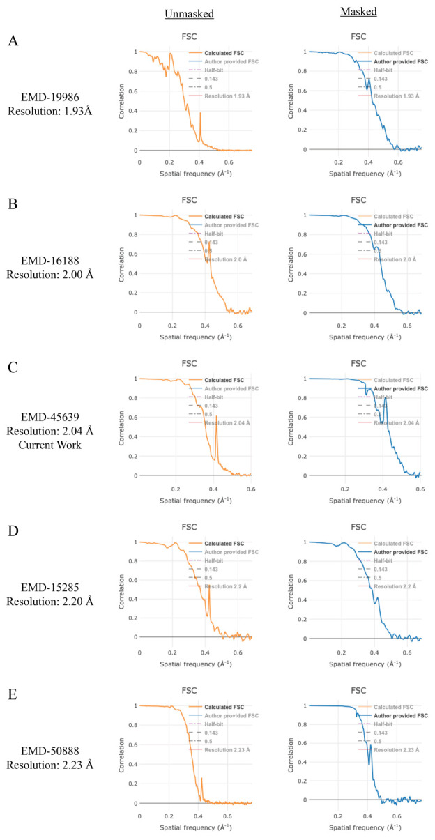
The unmasked FSC plots (calculated FSC from deposited half maps, orange) for the deposited maps display an FSC spike at a spatial frequency of 0.4 Å-1 (~2.4 Å). The masked FSC plots (author provided FSC, blue) dampen this feature.
46. Local resolution
Calculate a local resolution map to understand the differences in resolution across the map. Select the Local resolution job, set One of the 2 unfiltered half-maps to the run_half1_class001_unfil.mrc file from step 43, set User-provided solvent mask to the mask.mrc file from step 44, set the additional parameters below, and then click the Run! button.
I/O:
One of the 2 unfiltered half-maps: Refine3D/job107/run_half1_class001_unfil.mrc
User-provided solvent mask: MaskCreate/job109/mask.mrc
Calibrated pixel size (Å): 0.834
ResMap:
Use ResMap? No
Relion:
Use Relion? Yes
User-provided B-factor: -40
MTF of the detector (STAR file): k3-CDS-300keV-mtf.star
The job results in a histogram.pdf file that contains a graph of the local resolution within the provided mask. The relion_locres.mrc file can be opened in ChimeraX along with the postprocess.mrc file from step 45 to color the surface of the map by resolution (Figure 14). Please see the “Analyzing the results” section in the RELION local resolution documentation page for details on handling these maps in ChimeraX (https://relion.readthedocs.io/en/latest/SPA_tutorial/Validation.html).
Figure 14. Local resolution map of a-syn fibril from cryo-EM data.

A. Local resolution map of filamentous a-syn depicting a loss of resolution toward the end of the fibril, with the best resolution located along the central portion of the map. B. Cross-section of the local resolution map of filamentous a-syn showing that the best-resolved regions of the map are located along the fibril core and protofilament interface. Map resolution key spans from 1.8 Å (cyan) to 3.0 Å (red).
47. Real-space symmetrization (optional)
As stated previously, real-space symmetry is applied to only the central 25% of the reconstruction, and the molecular model is built into this central region (Figure 1E). However, in some cases, it is beneficial to extend the symmetrization to the edge of the box. For example, to better visualize the crossover distance, we generate a map with real-space symmetry imposed to the edge of the box, and then we align several models in ChimeraX to generate a multi-map volume that spans close to 1000 Å (Figure 1A). This process allows for easier visualization of the crossover distance when making figures. To impose real-space symmetry, run the relion_helix_toolbox command in the terminal. Before running the command, cd to the job directory for step 45.
relion_helix_toolbox --impose --i postprocess_masked.mrc --o postprocess_masked_sym.mrc --cyl_outer_diameter 220 --angpix 0.834 --rise 2.42 --twist 179.45 --z_percentage 0.25
The arguments used in the command above are as follows:
--impose apply real-space helical symmetry
--i input file
--o output file
--cyl_outer_diameter outer diameter of the cylindrical mask
--angpix pixel size in angstroms
--rise helical rise in angstroms
--twist helical twist in degrees
--z_percentage central z-length
F. Model building and validation for alpha-synuclein fibrils
There are many methods for building molecular models. Here, we used PDB 6H6B as a starting point; the model was fit into the EM map using ChimeraX and then one subunit was rebuilt and refined in Coot. The monomer model was subjected to a round of real-space refinement in Phenix. Then, ChimeraX was used to fit additional refined subunits into the map to generate a multimer model. The multimer model was subjected to a final round of real-space refinement in Phenix. We encourage users of this protocol to review tutorials and manuals for ChimeraX, Coot, and Phenix before proceeding with model building [41,42,46,50,51]. During the modeling process, users should use our refined model PDB 9CK3 as a reference. An overview of the entire modeling and validation workflow is provided for reference (Figure 15).
Figure 15. Model building and validation protocol for a-synuclein fibrils.

Step-by-step protocol for building, refining, and validating an a-syn fibril molecular model. This protocol uses ChimeraX, Coot, and Phenix in an iterative fashion to improve the molecular model.
1. Download PDB 6H6B by running open 6h6b from the ChimeraX command line [12]. This model covers residues 38–95 of the a-syn protein and contains 10 monomers displaying the amyloid fold.
2. Open the final postprocess.mrc file from step G45 and under Volume viewer set step size to 1.
3. In ChimeraX, use the Fit tool to place PDB 6H6B into the central region of the postprocess.mrc file. You may need to rotate the model to correctly fit the model into the map.
4. Run the command below from the ChimeraX command line to trim the ends of the map for easier visualization of the central region. Then, continue fitting until the model is well-placed on the map.
view orient; clip front -30 back 30
Note: Clipping can be turned off by running clip off from the ChimeraX command line.
5. Remove all but one monomer from the model by running split; delete #1.2–10 from the ChimeraX command line. We will use Coot to build and refine one subunit and add additional subunits later.
6. Save the file as a PDB, ensure that Save relative to model is checked, and select the post-processed map in the drop-down menu.
7. In Coot, go to File > Open Coordinates and select the PDB file saved in step 6. Then, go to File > Open Map and select the post-processed map from section G, step 45.
Note: We encourage new users to review the Coot tutorial to become familiar with the software before proceeding ( https://www2.mrc-lmb.cam.ac.uk/personal/pemsley/coot/web/tutorial/tutorial.pdf ).
8. On the right-hand side is the modeling toolbar; click Map, click Estimate to set the map weight, and then click Ok.
Note: Click the arrow at the bottom of the modeling toolbar and select Icons and text to add the name of each tool to the modeling toolbar.
9. Go to Refine > All-atom Refine to improve the fit of the map to the model. When the refinement is done, click Accept to save the refined atom positions. The refinement will impose geometry restraints and Ramachandran restraints but will ignore rotamers. We will handle rotamers in Phenix.
Note: Use the mouse scroll wheel to adjust the map contour level as necessary throughout this process.
10. The density generated in this protocol allows for the modeling of additional residues not resolved in PDB 6H6B, so we need to build additional regions of the model. Go to leucine 38, located at the n-terminus; from the modeling toolbar, click Add Terminal Residue and click on leucine 38. This will add an alanine residue to the n-terminus. From the modeling toolbar, click Simple Mutate, and then click on alanine 37. A window will appear listing all the amino acids; click Val (V) to change alanine 37 to a valine. From the modeling toolbar, click Real Space Refine Zone, then click on valine 37 and valine 40. This will refine the region between these two residues and improve the fit of the model to the map. Then, click Accept to save the refined atom positions.
11. Repeat step 10 to add glycine 36 to the n-terminus and lysine 96 and lysine 97 to the c-terminus.
12. Next, build residues 15–22 into a well-resolved island of density located near the n-terminus. Go to the island of density and rotate the density so the fibril core is oriented toward the top of the screen. This will help minimize the number of movements needed to place the strand into place. Go to Calculate > Other Modelling Tools > Place Strand Here, set Estimated number of residues in strand to 8 and click Go. A strand comprised of 8 alanine residues should now appear; use the Real Space Refine Zone tool to improve the fit of the strand into the map.
13. Use the Simple Mutate tool to change the alanine strand to the correct residues (V15, V16, A17, A18, A19, E20, K21, T22). Then, use the Real Space Refine Zone tool to further improve the fit of the strand.
Note: The n-terminus (i.e., island of density) folds back toward the fibril core adjacent to residues 36–44, with residue 15 closest to the fibril core.
14. Click on Display Manager and you will see that there are two molecules: one is the PDB that was imported and the second is the new strand that was created. We need to renumber the residues in the new strand, merge the molecules, and fix the chain ID. Go to Edit > Renumber Residues, under Renumber Residue Range of Molecule select the newly generated strand, under Start Residue select N-terminus, in the Apply Offset box provide an integer value to correct for the difference in residue number for the residue that should be valine 15, then click Apply. For example, if the valine on the n-terminus of the strand is labeled as V40, then the offset should be -25 to set the valine to residue 15. Click on the n-terminus valine of the strand to verify the numbering is correct.
15. To merge the molecules, Go to Edit > Merge Molecules, under Append/Insert Molecule(s) select the strand, and under into Molecule select the original PDB from the drop-down menu. Then, click Merge.
16. Change the chain IDs so both fragments are labeled as chain A. Go to Edit > Change Chain IDs, under Change Chain ID in Molecule select the file that contains both fragments (i.e., the recently merged molecule), under From Chain ID select either chain, under Using Residue Selection select Whole Chain, under To Chain ID set this value to A, then click Apply New Chain ID. Repeat the process if the second fragment is labeled anything other than chain A. The fragments should now be one molecule labeled as chain A with a dotted line showing the missing residues from residues 23 to 35 that are not resolved.
17. Refine the new molecule that spans residues 15–22 and 36–97 (Figure 16). Go to Refine > All-atom Refine and, if the atoms are well-positioned, click Accept. If not, manually adjust misplaced atoms by dragging the atoms into place and then click Accept.
Figure 16. a-synuclein map and model.

A cross-section shows the molecular model and the cryo-EM map shows excellent agreement. Side-chain densities are clear and allow for modeling residues V15–T22 and G36–K97. Scale bar, 25 Å.
18. Save the coordinates, go to File > Save Coordinates, under Select Molecule Number to Save select the molecules that were refined in step 17, click Select Filename, and save the file to the desired location.
19. Open Phenix and set up a new project.
Note: We encourage new users to review the Phenix tutorial, specifically the real space refinement tutorial, to become familiar with the software before proceeding ( https://phenix-online.org/documentation/reference/real_space_refine.html ).
20. Under the cryo-EM section, select the Real-space refinement job. Provide the PDB file from Coot as the model file and the post-processed file as the map file. Set Resolution as determined in the final RELION post-processing job; in this case, the resolution is 2.04 Å. Under the Refinement Settings tab, in addition to the default settings, ensure Use secondary structure restraints and Ramachandran restraints is checked, set Nproc to 4, click Rotamers, and under Fit, select outliers and poormap, then click Run. Upon completion, the validation report shows that the model statistics are favorable. The Rotamer outliers (%) will be slightly elevated due to a salt bridge that forms between lysine 80 and glutamic acid 46, causing lysine 80 to be a rotamer outlier that is supported by the data.
21. In ChimeraX, open the refined model and the post-processed map. Open the refined model again; now, two models are available. Select the second model and use the Fit tool to place the second monomer into the opposing protofilament. Repeat the process of opening the refined model and fitting it into a new region of the map. For PDB 9CK3, we built a dodecamer model.
22. Once the desired number of subunits are fitted into the map, run combine from the ChimeraX command line to merge the subunits into one model. The command should provide a unique chain ID to each subunit.
23. Repeat step F6 to save the model relative to the post-processed map.
24. In Phenix, repeat real space refinement as in step 20 with the additional parameter Ncs constraints selected. The final validation report shows excellent model statistics with only lysine 80 as a rotamer outlier, as expected (Table 1). This step can be repeated, if necessary. The model is now ready for structure analysis.
Table 1. Data collection, reconstruction, and model statistics.
| Protein | a-syn (apo) fibrils |
|---|---|
| PDB ID | 9CK3 |
| EMDB ID | EMD-45639 |
| Data collection and processing | |
| Voltage (kV) | 300 |
| Electron exposure (e-/Å2) | 40 |
| Number of frames | 40 |
| Nominal defocus range (-mm) | 0.5–2.5, 0.25 step |
| Pixel size (Å) | 0.834 |
| Symmetry (beyond helical) | C 1 |
| Micrographs | 5,193 |
| Final particles | 129,895 |
| Box size (Å) | 300 |
| Box size (pixels) | 360 |
| Helical symmetry | |
| rise (Å) | 2.42 |
| twist (°) | 179.45 |
| Helical Z parameter (%) | |
| masking | 25 |
| refinement | 25 |
| Map resolution (Å) threshold | 0.143 |
| Masked | 2.04 |
| Unmasked | 2.35 |
| Sharpening B factor (Å2) | -43 |
| Structure Refinement | |
| Total atoms | 5,748 |
| ligands | 0 |
| water | 0 |
| RMS, bonds (Å) | 0.004 |
| RMS, angles (o) | 0.643 |
| Ramachandran favored (%) | 98.48 |
| Ramachandran outliers (%) | 0.00 |
| Rotamer outliers (%) | 2.08 |
| Map-model correlation (masked) | 0.90 |
| Model B factors | |
| minimum | 5.38 |
| mean | 41.28 |
| maximum | 88.56 |
| MolProbity score | 1.42 |
| Clashscore | 3.88 |
Data analysis
Cryo-EM data processing depends on the sample, data collection instrumentation and parameters used, and computational hardware and software. The workflow presented here should provide users with the necessary details for cryo-EM structure determination of amyloid fibrils. The protocol presented here was used to generate a cryo-EM map and atomic model of in vitro–assembled a-syn fibrils. Atomic models have been deposited in the Protein Data Bank (PDB) under accession 9CK3. Cryo-EM maps, including the final map, half-maps, and mask have been deposited in the Electron Microscopy Data Bank (EMDB) under accession EMD-45639.
Validation of protocol
This protocol or parts of it has been used and validated in the following research articles:
• Dhavale et al. [33]. Structure of alpha-synuclein fibrils derived from human Lewy boy dementia tissue. Nature Communications. https://doi.org/10.1038/s41467-024-46832-5.
• Montemayor et al. [52]. Flagellar Structures from the Bacterium Caulobacter crescentus and Implications for Phage φ CbK Predation of Multiflagellin Bacteria. Journal of Bacteriology. https://doi.org/10.1128/jb.00399-20.
• Sanchez et al. [53]. Atomic-level architecture of Caulobacter crescentus flagellar filaments provide evidence for multi-flagellin filament stabilization. bioRxiv. https://doi.org/10.1101/2023.07.10.548443.
• The cryo-EM structure in the manuscript has been validated by our submissions to the PDB (9CK3) and EMDB (EMD-45639). https://doi.org/10.2210/pdb9CK3/pdb.
Limitations
The fibrilization conditions presented here are specific to one form of in vitro–assembled a-syn fibrils. Extensive optimization of protein purification and fibrilization conditions, testing buffer conditions, and incubation parameters may be necessary to generate different in vitro forms. The cryo-EM helical reconstruction methods presented here assume that fibrils are both twisting and of sufficient length to determine the crossover distance for helical twist estimates. There are cases where fibrils may not twist, and thus, this workflow would not be amendable to such samples. Finally, structure determination of patient-derived fibrils is of high interest, but extraction of fibrils from patient tissue is outside of the scope of the work presented here. Though, in theory, the data processing methods presented here should be applicable to these samples.
General notes and troubleshooting
Troubleshooting
The workflow presented here, including sample preparation, NS-TEM, cryo-EM data collection, cryo-EM data processing, and molecular model building, serves as a starting point for individuals new to cryo-EM structural analyses of amyloid proteins. For cryo-EM structure determination, new samples will pose their own unique set of challenges, but by first completing the data processing workflow in section E with the EMPIAR-12229 dataset under accession EMPIAR-12229, new users will be more adept at troubleshooting new issues.
Acknowledgments
This work was supported in part by the University of Wisconsin, Madison, the Department of Biochemistry at the University of Wisconsin, Madison, and public health service grants U24 GM139168 to E.R.W, P41GM136463 to C.M.R, and RF1 NS110436 E.R.W. and C.M.R. from the NIH. J.C.S. was supported in part by the Biotechnology Training Program at the University of Wisconsin, Madison, T32 GM135066, the Steenbock Predoctoral Graduate Fellowship administered by the University of Wisconsin-Madison Department of Biochemistry, and the SciMed Graduate Research Scholars Fellowship with support for this fellowship provided by the Graduate School, part of the Office of Vice Chancellor for Research and Graduate Education at the University of Wisconsin-Madison, with funding from the Wisconsin Alumni Research Foundation and the UW-Madison. C.G.B. was supported by the NIH Ruth L. Kirschstein Fellowship, F32 GM149118, from the NIGMS. We are grateful for the critical feedback, guidance, and support provided by Dr. Bryan Sibert, Dr. Matthew Larson, and Ms. Jennifer Scheuren on cryo-EM data collection, data processing, and use of the cryo-EM HPC cluster. We are grateful to Mr. Owen Warmuth for assistance with the SDS-PAGE gel image. We are grateful for the use of facilities and instrumentation at the Cryo-EM Research Center in the Department of Biochemistry at the University of Wisconsin, Madison. We are grateful for the computational resources supplied through the SBGrid Consortium [34].
Data deposition
The atomic model was deposited in the Protein Data Bank under accession 9CK3. Cryo-EM maps were deposited in the Electron Microscopy Data Bank under accession EMD-45639. The raw micrographs, gain file, and detector MTF file are available on the EMPIAR-12229 database under accession EMPIAR-12229.
Competing interests
The authors declare no competing interests.
References
- 1. Baba M., Nakajo S., Tu P. H., Tomita T., Nakaya K., Lee V. M., Trojanowski J. Q., Iwatsubo T.(1998). Aggregation of alpha-synuclein in Lewy bodies of sporadic Parkinson's disease and dementia with Lewy bodies. Am J Pathol. 152: 879-884. [PMC free article] [PubMed] [Google Scholar]
- 2. Spillantini M. G., Schmidt M. L., Lee V. M., Trojanowski J. Q., Jakes R. and Goedert M.(1997). Alpha-synuclein in Lewy bodies. Nature. 388(6645): 839-840. [DOI] [PubMed] [Google Scholar]
- 3. Tu P., Galvin J. E., Baba M., Giasson B., Tomita T., Leight S., Nakajo S., Iwatsubo T., Trojanowski J. Q., Lee V. M., et al.(1998). Glial cytoplasmic inclusions in white matter oligodendrocytes of multiple system atrophy brains contain insoluble α‐synuclein. Ann Neurol. 44(3): 415-422. [DOI] [PubMed] [Google Scholar]
- 4. Eisenberg D. S. and Sawaya M. R.(2017). Structural Studies of Amyloid Proteins at the Molecular Level. Annu Rev Biochem. 86(1): 69-95. [DOI] [PubMed] [Google Scholar]
- 5. Burré J., Sharma M., Tsetsenis T., Buchman V., Etherton M. R. and Südhof T. C.(2010). α-Synuclein Promotes SNARE-Complex Assembly in Vivo and in Vitro. Science. 329(5999): 1663-1667. [DOI] [PMC free article] [PubMed] [Google Scholar]
- 6. Davidson W. S., Jonas A., Clayton D. F. and George J. M.(1998). Stabilization of α-Synuclein Secondary Structure upon Binding to Synthetic Membranes. J Biol Chem. 273(16): 9443-9449. [DOI] [PubMed] [Google Scholar]
- 7. Lou X., Kim J., Hawk B. J. and Shin Y. K.(2017). α-Synuclein may cross-bridge v-SNARE and acidic phospholipids to facilitate SNARE-dependent vesicle docking. Biochem J. 474(12): 2039-2049. [DOI] [PMC free article] [PubMed] [Google Scholar]
- 8. Sun J., Wang L., Bao H., Premi S., Das U., Chapman E. R. and Roy S.(2019). Functional cooperation of α-synuclein and VAMP2 in synaptic vesicle recycling. Proc Natl Acad Sci USA. 116(23): 11113-11115. [DOI] [PMC free article] [PubMed] [Google Scholar]
- 9. Thapa K., Khan H., Kanojia N., Singh T. G., Kaur A. and Kaur G.(2022). Therapeutic Insights on Ferroptosis in Parkinson's disease. Eur J Pharmacol. 930: 175133. [DOI] [PubMed] [Google Scholar]
- 10. Serpell L. C., Berriman J., Jakes R., Goedert M. and Crowther R. A.(2000). Fiber diffraction of synthetic α-synuclein filaments shows amyloid-like cross-β conformation. Proc Natl Acad Sci USA. 97(9): 4897-4902. [DOI] [PMC free article] [PubMed] [Google Scholar]
- 11. Spillantini M. G., Goedert M.(2000). The alpha-synucleinopathies: Parkinson's disease, dementia with Lewy bodies, and multiple system atrophy. Ann N Y Acad Sci. 920(1): 16-27. [DOI] [PubMed] [Google Scholar]
- 12. Guerrero-Ferreira R., Taylor N. M., Mona D., Ringler P., Lauer M. E., Riek R., Britschgi M. and Stahlberg H.(2018). Cryo-EM structure of alpha-synuclein fibrils. eLife. 7: e36402. [DOI] [PMC free article] [PubMed] [Google Scholar]
- 13. Li Y., Zhao C., Luo F., Liu Z., Gui X., Luo Z., Zhang X., Li D., Liu C., Li X., et al.(2018). Amyloid fibril structure of α-synuclein determined by cryo-electron microscopy. Cell Res. 28(9): 897-903. [DOI] [PMC free article] [PubMed] [Google Scholar]
- 14. Tuttle M. D., Comellas G., Nieuwkoop A. J., Covell D. J., Berthold D. A., Kloepper K. D., Courtney J. M., Kim J. K., Barclay A. M., Kendall A., et al.(2016). Solid-state NMR structure of a pathogenic fibril of full-length human α-synuclein. Nat Struct Mol Biol. 23(5): 409-415. [DOI] [PMC free article] [PubMed] [Google Scholar]
- 15. Lei Z., Cao G. and Wei G.(2019). A30P mutant α-synuclein impairs autophagic flux by inactivating JNK signaling to enhance ZKSCAN3 activity in midbrain dopaminergic neurons. Cell Death Dis. 10(2): 133. [DOI] [PMC free article] [PubMed] [Google Scholar]
- 16. Zarranz J. J., Alegre J., Gómez‐Esteban J. C., Lezcano E., Ros R., Ampuero I., Vidal L., Hoenicka J., Rodriguez O., Atarés B., et al.(2003). The new mutation, E46K, of α‐synuclein causes parkinson and Lewy body dementia. Ann Neurol. 55(2): 164-173. [DOI] [PubMed] [Google Scholar]
- 17. Appel-Cresswell S., Vilarino-Guell C., Encarnacion M., Sherman H., Yu I., Shah B., Weir D., Thompson C., Szu-Tu C., Trinh J., et al.(2013). Mov Disord. 28(6): 811–813. [DOI] [PubMed]
- 18. Lesage S., Anheim M., Letournel F., Bousset L., Honoré A., Rozas N., Pieri L., Madiona K., Dürr A., Melki R., et al.(2013). G51D α‐synuclein mutation causes a novel Parkinsonian–pyramidal syndrome. Ann Neurol. 73(4): 459-471. [DOI] [PubMed] [Google Scholar]
- 19. Pasanen P., Myllykangas L., Siitonen M., Raunio A., Kaakkola S., Lyytinen J., Tienari P. J., Pöyhönen M. and Paetau A.(2014). A novel α-synuclein mutation A53E associated with atypical multiple system atrophy and Parkinson's disease-type pathology. Neurobiol Aging. 35(9): 2180 .e1–2180.e5. [DOI] [PubMed] [Google Scholar]
- 20. Polymeropoulos M. H., Lavedan C., Leroy E., Ide S. E., Dehejia A., Dutra A., Pike B., Root H., Rubenstein J., Boyer R., et al.(1997). Mutation in the α-Synuclein Gene Identified in Families with Parkinson's Disease. Science. 276(5321): 2045-2047. [DOI] [PubMed] [Google Scholar]
- 21. Yoshino H., Hirano M., Stoessl A. J., Imamichi Y., Ikeda A., Li Y., Funayama M., Yamada I., Nakamura Y., Sossi V., et al.(2017). Homozygous alpha-synuclein p.A53V in familial Parkinson's disease. Neurobiol Aging. 57: 248 .e7–248.e12. [DOI] [PubMed] [Google Scholar]
- 22. Frey L., Ghosh D., Qureshi B. M., Rhyner D., Guerrero-Ferreira R., Pokharna A., Kwiatkowski W., Serdiuk T., Picotti P., Riek R., et al.(2024). On the pH-dependence of α-synuclein amyloid polymorphism and the role of secondary nucleation in seed-based amyloid propagation. eLife. 12: e93562. [DOI] [PMC free article] [PubMed] [Google Scholar]
- 23. Mehra S., Gadhe L., Bera R., Sawner A. S. and Maji S. K.(2021). Structural and Functional Insights into α-Synuclein Fibril Polymorphism. Biomolecules. 11(10): 1419. [DOI] [PMC free article] [PubMed] [Google Scholar]
- 24. Peelaerts W., Bousset L., Van der Perren A., Moskalyuk A., Pulizzi R., Giugliano M., Van den Haute C., Melki R. and Baekelandt V.(2015). α-Synuclein strains cause distinct synucleinopathies after local and systemic administration. Nature. 522(7556): 340-344. [DOI] [PubMed] [Google Scholar]
- 25. Marotta N. P., Ara J., Uemura N., Lougee M. G., Meymand E. S., Zhang B., Petersson E. J., Trojanowski J. Q. and Lee V. Y.(2021). Alpha-synuclein from patient Lewy bodies exhibits distinct pathological activity that can be propagated in vitro. Acta Neuropathol Commun. 9(1): 188. [DOI] [PMC free article] [PubMed] [Google Scholar]
- 26. Uemura N., Marotta N. P., Ara J., Meymand E. S., Zhang B., Kameda H., Koike M., Luk K. C., Trojanowski J. Q., Lee V. Y., et al.(2023). α-Synuclein aggregates amplified from patient-derived Lewy bodies recapitulate Lewy body diseases in mice. Nat Commun. 14(1): 6892. [DOI] [PMC free article] [PubMed] [Google Scholar]
- 27. Yang Y., Shi Y., Schweighauser M., Zhang X., Kotecha A., Murzin A. G., Garringer H. J., Cullinane P. W., Saito Y., Foroud T., et al.(2022). Structures of α-synuclein filaments from human brains with Lewy pathology. Nature. 610(7933): 791-795. [DOI] [PMC free article] [PubMed] [Google Scholar]
- 28. Riek R. and Eisenberg D. S.(2016). The activities of amyloids from a structural perspective. Nature. 539(7628): 227-235. [DOI] [PubMed] [Google Scholar]
- 29. Jarrett J. T. and Lansbury P. T.(1992). Amyloid fibril formation requires a chemically discriminating nucleation event: studies of an amyloidogenic sequence from the bacterial protein OsmB. Biochemistry. 31(49): 12345-12352. [DOI] [PubMed] [Google Scholar]
- 30. Törnquist M., Michaels T. C. T., Sanagavarapu K., Yang X., Meisl G., Cohen S. I. A., Knowles T. P. J. and Linse S.(2018). Secondary nucleation in amyloid formation. Chem Commun. 54(63): 8667-8684. [DOI] [PubMed] [Google Scholar]
- 31. Tanaka G., Yamanaka T., Furukawa Y., Kajimura N., Mitsuoka K. and Nukina N.(2019). Sequence- and seed-structure-dependent polymorphic fibrils of alpha-synuclein. BBA Mol Basis Dis. 1865(6): 1410-1420. [DOI] [PubMed] [Google Scholar]
- 32. Strohäker T., Jung B. C., Liou S. H., Fernandez C. O., Riedel D., Becker S., Halliday G. M., Bennati M., Kim W. S., Lee S. J., et al.(2019). Structural heterogeneity of α-synuclein fibrils amplified from patient brain extracts. Nat Commun. 10(1): 5535. [DOI] [PMC free article] [PubMed] [Google Scholar]
- 33. Dhavale D. D., Barclay A. M., Borcik C. G., Basore K., Berthold D. A., Gordon I. R., Liu J., Milchberg M. H., O’Shea J. Y., Rau M. J., et al.(2024). Structure of alpha-synuclein fibrils derived from human Lewy body dementia tissue. Nat Commun. 15(1): 2750. [DOI] [PMC free article] [PubMed] [Google Scholar]
- 34. Morin A., Eisenbraun B., Key J., Sanschagrin P. C., Timony M. A., Ottaviano M. and Sliz P.(2013). Collaboration gets the most out of software. eLife. 2: e01456. [DOI] [PMC free article] [PubMed] [Google Scholar]
- 35. Kremer J. R., Mastronarde D. N. and McIntosh J.(1996). Computer Visualization of Three-Dimensional Image Data Using IMOD. J Struct Biol. 116(1): 71-76. [DOI] [PubMed] [Google Scholar]
- 36. Kimanius D., Dong L., Sharov G., Nakane T. and Scheres S. H. W.(2021). New tools for automated cryo-EM single-particle analysis in RELION-4.0. Biochem J. 478(24): 4169-4185. [DOI] [PMC free article] [PubMed] [Google Scholar]
- 37. Scheres S. H.(2012). RELION: Implementation of a Bayesian approach to cryo-EM structure determination. J Struct Biol. 180(3): 519-530. [DOI] [PMC free article] [PubMed] [Google Scholar]
- 38. Zheng S. Q., Palovcak E., Armache J. P., Verba K. A., Cheng Y. and Agard D. A.(2017). MotionCor2: anisotropic correction of beam-induced motion for improved cryo-electron microscopy. Nat Methods. 14(4): 331-332. [DOI] [PMC free article] [PubMed] [Google Scholar]
- 39. Zhang K.(2016). Gctf: Real-time CTF determination and correction. J Struct Biol. 193(1): 1-12. [DOI] [PMC free article] [PubMed] [Google Scholar]
- 40. Bepler T., Morin A., Rapp M., Brasch J., Shapiro L., Noble A. J. and Berger B.(2019). Positive-unlabeled convolutional neural networks for particle picking in cryo-electron micrographs. Nat Methods. 16(11): 1153-1160. [DOI] [PMC free article] [PubMed] [Google Scholar]
- 41. Pettersen E. F., Goddard T. D., Huang C. C., Meng E. C., Couch G. S., Croll T. I., Morris J. H. and Ferrin T. E.(2020). UCSF ChimeraX: Structure visualization for researchers, educators, and developers. Protein Sci. 30(1): 70-82. [DOI] [PMC free article] [PubMed] [Google Scholar]
- 42. Goddard T. D., Huang C. C., Meng E. C., Pettersen E. F., Couch G. S., Morris J. H. and Ferrin T. E.(2017). UCSF ChimeraX: Meeting modern challenges in visualization and analysis. Protein Sci. 27(1): 14-25. [DOI] [PMC free article] [PubMed] [Google Scholar]
- 43. Afonine P. V., Poon B. K., Read R. J., Sobolev O. V., Terwilliger T. C., Urzhumtsev A. and Adams P. D.(2018). Real-space refinement inPHENIXfor cryo-EM and crystallography. Acta Crystallogr D Struct Biol. 74(6): 531-544. [DOI] [PMC free article] [PubMed] [Google Scholar]
- 44. Naiki H., Higuchi K., Hosokawa M. and Takeda T.(1989). Fluorometric determination of amyloid fibrils in vitro using the fluorescent dye, thioflavine T. Anal Biochem. 177(2): 244-249. [DOI] [PubMed] [Google Scholar]
- 45. Scheres S. H. W.(2020). Amyloid structure determination in RELION-3.1. Acta Crystallogr D Struct Biol. 76(2): 94-101. [DOI] [PMC free article] [PubMed] [Google Scholar]
- 46. Meng E. C., Goddard T. D., Pettersen E. F., Couch G. S., Pearson Z. J., Morris J. H. and Ferrin T. E.(2023). UCSF ChimeraX: Tools for structure building and analysis. Protein Sci. 32(11): e4792. [DOI] [PMC free article] [PubMed] [Google Scholar]
- 47. Fitzpatrick A. W. P., Falcon B., He S., Murzin A. G., Murshudov G., Garringer H. J., Crowther R. A., Ghetti B., Goedert M., Scheres S. H. W., et al.(2017). Cryo-EM structures of tau filaments from Alzheimer’s disease. Nature. 547(7662): 185-190. [DOI] [PMC free article] [PubMed] [Google Scholar]
- 48. Yang Y., Garringer H. J., Shi Y., Lövestam S., Peak-Chew S., Zhang X., Kotecha A., Bacioglu M., Koto A., Takao M., et al.(2023). New SNCA mutation and structures of α-synuclein filaments from juvenile-onset synucleinopathy. Acta Neuropathol. 145(5): 561-572. [DOI] [PMC free article] [PubMed] [Google Scholar]
- 49. Egelman E. H.(2024). Helical reconstruction, again. Curr Opin Struct Biol. 85: 102788. [DOI] [PMC free article] [PubMed] [Google Scholar]
- 50. Emsley P., Lohkamp B., Scott W. G. and Cowtan K.(2010). Features and development of Coot . Acta Crystallogr D Biol Crystallogr. 66(4): 486-501. [DOI] [PMC free article] [PubMed] [Google Scholar]
- 51. Liebschner D., Afonine P. V., Baker M. L., Bunkóczi G., Chen V. B., Croll T. I., Hintze B., Hung L. W., Jain S., McCoy A. J., et al.(2019). Macromolecular structure determination using X-rays, neutrons and electrons: recent developments in Phenix . Acta Crystallogr D Struct Biol. 75(10): 861-877. [DOI] [PMC free article] [PubMed] [Google Scholar]
- 52. Montemayor E. J., Ploscariu N. T., Sanchez J. C., Parrell D., Dillard R. S., Shebelut C. W., Ke Z., Guerrero-Ferreira R. C. and Wright E. R.(2021). Flagellar Structures from the Bacterium Caulobacter crescentus and Implications for Phage ϕ CbK Predation of Multiflagellin Bacteria. J Bacteriol. 203(5): e00399-20. [DOI] [PMC free article] [PubMed] [Google Scholar]
- 53. Sanchez J. C., Montemayor E. J., Ploscariu N. T., Parrell D., Baumgardt J. K., Yang J. E., Sibert B., Cai K. and Wright E. R.(2023). Atomic-level architecture of Caulobacter crescentus flagellar filaments provide evidence for multi-flagellin filament stabilization. bioRxiv. doi.org/ 10.1101/2023.07 .10.548443. [DOI] [Google Scholar]