Recent advances in deep learning have triggered a variety of business applications based on computer vision. There are many industry segments where deep learning tools and techniques are applied in object recognition in order to make the business process much faster. The apparel industry is one among them. By presenting the image of any apparel, the trained deep learning model can predict the name of that apparel and this process can be repeated at a very much faster speed in order to tag thousands of apparels in very less time with high accuracy. 

In this article, we will discuss fashion apparel recognition using the Convolutional Neural Network (CNN) model. To train the CNN model, we will use the Fashion MNIST dataset. After successful training, the CNN model can predict the name of the class a given apparel item belongs to. This is a multiclass classification problem in which there are 10 apparel classes the items will be classified.

The Data Set

In this article, we have used the Fashion MNIST data set that is publicly available on Kaggle. It consists of a training set of 60,000 example images and a test set of 10,000 example images. Each image in the dataset has the size 28 x 28 pixels. Each training and test image belongs to one of the classes including T_shirt/top, Trouser, Pullover, Dress, Coat, Sandal, Shirt, Sneaker, Bag, and Ankle boot. The original training and test image data sets are converted into CSV files and made available on Kaggle. 

Implementation

This execution is done in Google Colab and to read the CSV files there, we first uploaded the CSV files to Google Drive and then mounted the drive using the following lines of codes. 

#Setting google drive as a directory for dataset
from google.colab import drive 
drive.mount('/content/gdrive')

Once Google Drive is mounted, we will read our training and test CSV files using the below lines of codes.

#Reading dataset
import pandas as pd 
fashion_train_df = pd.read_csv('gdrive/My Drive/fashion-mnist_train.csv',sep=',')
fashion_test_df = pd.read_csv('gdrive/My Drive/fashion-mnist_test.csv', sep = ',')

After successfully reading the data sets, we will import the other required libraries. 

#Importing other required libraries
import pandas as pd 
import numpy as np 
import matplotlib.pyplot as plt 
import seaborn as sns
import random
sns.set_style("whitegrid")

The data sets that we have read above, we will see their shapes. As we discussed earlier, there are 60,000 examples in the training set and 10,000 examples in the test set. 

#Shape of training data
fashion_train_df.shape



#Shape of test data
fashion_test_df.shape

Since the size of each image is 28 x 28 hence there are a total of 784 pixels of each image and there is one column of class label. That is why a total of 785 columns are there in the dataset. 

Now, in order to define the training and test data sets, first, we need to create the training and test arrays. 

# Create training and testing arrays
train = np.array(fashion_train_df, dtype = 'float32')
test = np.array(fashion_test_df, dtype='float32')

The below line of code specifies the class labels of the data set, as given in the description on Kaggle. 

#Specifying class labels
class_names = ['T_shirt/top', 'Trouser', 'Pullover', 'Dress', 'Coat', 'Sandal', 'Shirt', 'Sneaker', 'Bag', 'Ankle boot']

Now, to proceed further and validating the class label, we will pick and plot a random image from the set of 60,000 training images to verify its correct class label. The below lines of codes can pick and plot a different image randomly in each run.

#See a random image for class label verification
i = random.randint(1,60000)
plt.imshow(train[i,1:].reshape((28,28))) 

plt.imshow(train[i,1:].reshape((28,28)) , cmap = 'gray') 
label_index = fashion_train_df["label"][i]
plt.title(f"{class_names[label_index]}")
plt.axis('off')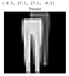

To verify the same, we will see the class label of the above randomly selected image and match the label with the label name.

#Label of the random image
label = train[i,0]
label

As we are confirmed about the class label and class name with one randomly selected image, now will visualize more random images with class labels and class names. The number of images to be chosen can be adjusted by changing the values of width and length grid W_grid and L_grid respectively. We could use subplot but it returns the figure object and axes object. Here, we can use the axes object to plot specific figures at various locations.

# Define the dimensions of the plot grid 
W_grid = 15
L_grid = 15
fig, axes = plt.subplots(L_grid, W_grid, figsize = (17,17))
axes = axes.ravel() # flaten the 15 x 15 matrix into 225 array
n_train = len(train) # get the length of the train dataset
# Select a random number from 0 to n_train
for i in np.arange(0, W_grid * L_grid): # create evenly spaces variables 
    # Select a random number
    index = np.random.randint(0, n_train)
    # read and display an image with the selected index    
    axes[i].imshow( train[index,1:].reshape((28,28)) )
    label_index = int(train[index,0])
    axes[i].set_title(class_names[label_index], fontsize = 8)
    axes[i].axis('off')
plt.subplots_adjust(hspace=0.4)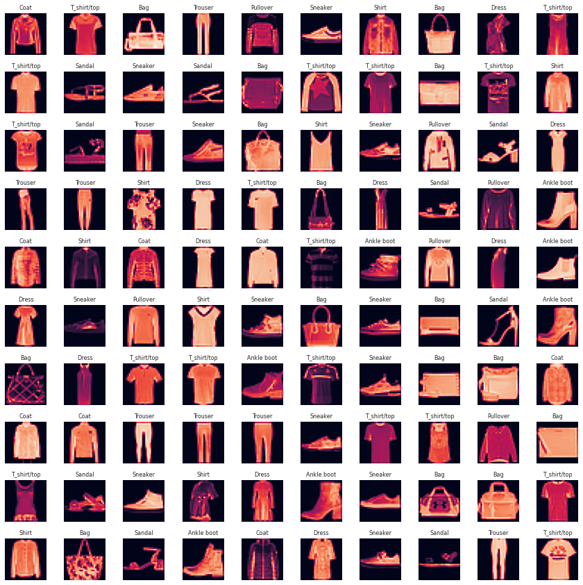

We can run the above set of codes to verify class name for images. In each run, a random set of images will be visualized. Now we are correct with the class labels and names of all the images.

In the next step, we will prepare the training and test data.

# Prepare the training and testing dataset 
X_train = train[:, 1:] / 255
y_train = train[:, 0]

X_test = test[:, 1:] / 255
y_test = test[:,0]

We will visualize a set of 25 training image data that will be used to train the convolutional neural network model.

plt.figure(figsize=(10, 10))
for i in range(25):
    plt.subplot(5, 5, i + 1)
    plt.xticks([])
    plt.yticks([])
    plt.grid(False)
    plt.imshow(X_train[i].reshape((28,28)), cmap=plt.cm.binary)
    label_index = int(y_train[i])
    plt.title(class_names[label_index])
plt.show()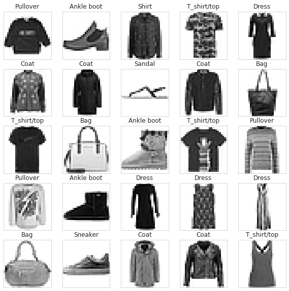

For the training and validation purpose, we split the data set accordingly. The test data size can be adjusted after a run of the model. 

#Split the training and test sets
from sklearn.model_selection import train_test_split
X_train, X_validate, y_train, y_validate = train_test_split(X_train, y_train, test_size = 0.2, random_state = 12345)

print(X_train.shape)
print(y_train.shape)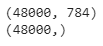

Here, we will unfold the data to make it available for training, testing and validation purpose.

# Unpack the training and test tuple
X_train = X_train.reshape(X_train.shape[0], *(28, 28, 1))
X_test = X_test.reshape(X_test.shape[0], *(28, 28, 1))
X_validate = X_validate.reshape(X_validate.shape[0], *(28, 28, 1))

print(X_train.shape)
print(y_train.shape)
print(X_validate.shape)

To define and train the convolutional neural network, we will import the required libraries here.

#Library for CNN Model
import keras
from keras.models import Sequential
from keras.layers import Conv2D, MaxPooling2D, Dense, Flatten, Dropout
from keras.optimizers import Adam
from keras.callbacks import TensorBoard

Convolutional Neural Network

In the below line of codes, we will define our convolutional neural network model. For more understanding about the convolutional neural network, please refer to the article ‘Overview of Convolutional Neural Network in Image Classification’.

#Defining the Convolutional Neural Network
cnn_model = Sequential()

cnn_model.add(Conv2D(32, (3, 3), input_shape = (28,28,1), activation='relu'))
cnn_model.add(MaxPooling2D(pool_size = (2, 2)))
cnn_model.add(Dropout(0.25))

cnn_model.add(Conv2D(64, (3, 3), input_shape = (28,28,1), activation='relu'))
cnn_model.add(MaxPooling2D(pool_size = (2, 2)))
cnn_model.add(Dropout(0.25))

cnn_model.add(Conv2D(128, (3, 3), input_shape = (28,28,1), activation='relu'))
cnn_model.add(MaxPooling2D(pool_size = (2, 2)))
cnn_model.add(Dropout(0.25))

cnn_model.add(Flatten())
cnn_model.add(Dense(units = 512, activation = 'relu'))
cnn_model.add(Dropout(0.25))
cnn_model.add(Dense(units = 10, activation = 'softmax'))

cnn_model.summary()

After defining the CNN model and viewing its summary, we will bind-up this model by compiling it.

#Compiling
cnn_model.compile(loss ='sparse_categorical_crossentropy', optimizer='adam' ,metrics =['accuracy'])

In the next step, we will train our CNN model on the image classification. The below hyperparameters can be tuned for better accuracy of the model.

#Training the CNN model
history = cnn_model.fit(X_train, y_train, batch_size = 512, epochs = 200, verbose = 1, validation_data = (X_validate, y_validate))

After successful training, we will visualize the loss and accuracy of the model through a plot using below lines of codes.

#VIsualizing the training performance
plt.figure(figsize=(12, 8))

plt.subplot(2, 2, 1)
plt.plot(history.history['loss'], label='Loss')
plt.plot(history.history['val_loss'], label='val_Loss')
plt.legend()
plt.title('Loss evolution')

plt.subplot(2, 2, 2)
plt.plot(history.history['accuracy'], label='accuracy')
plt.plot(history.history['val_accuracy'], label='val_accuracy')
plt.legend()
plt.title('Accuracy evolution')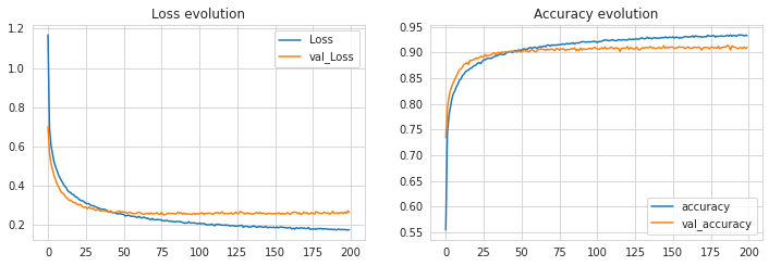

We could perform training in multiple iterations by tuning the hyperparameters to see an increase in the accuracy of the model. But we found this consistent level with these values of hyperparameter and 200 epochs of training.

As the model is trained successfully and we could achieve an accuracy of more than 93% during training and more than 90% during validations, we consider this CNN model as best fitted with our data. So now will make predictions using this CNN model on test data. The model is expected to produce class labels as the output of prediction. 

#Predictions for the test data
predicted_classes = cnn_model.predict_classes(X_test)

test_img = X_test[0]
prediction = cnn_model.predict(test_img)
prediction[0]


np.argmax(prediction[0])

As we can see above that the model has predicted the class label 0 for the given image. Now, we will check the prediction on more images. We are taking 49 images as a test set and predicting their class labels and comparing the predicted class labels with true class labels.

L = 7
W = 7
fig, axes = plt.subplots(L, W, figsize = (18,18))
axes = axes.ravel()

for i in np.arange(0, L * W):  
    axes[i].imshow(X_test[i].reshape(28,28))
    axes[i].set_title(f"Prediction Class = {predicted_classes[i]:0.1f}\n True Class = {y_test[i]:0.1f}")
    axes[i].axis('off')
plt.subplots_adjust(wspace=0.5)

For the window limitation, we have taken only 7 x 7 = 49 images, but one can take more images to predict class labels. As we can see in the above visualization, for all 49 images, our CNN model has predicted correct class labels for 45 images and incorrect class labels for 4 images.

For better understanding, let us visualize the total classification done by the model using confusion matrices. For better visualization of the confusion matrix, first, we will define the class labels and then create the confusion matrix.

class_names = ['T_shirt/top', 'Trouser', 'Pullover', 'Dress', 'Coat', 'Sandal', 'Shirt', 'Sneaker', 'Bag', 'Ankle boot']

from sklearn.metrics import confusion_matrix
from sklearn import metrics
cm = metrics.confusion_matrix(y_test, predicted_classes)

For better visualization of the confusion matrix, a function ‘plot_confusion_matrix’ is being used here.

#Defining function for confusion matrix plot
def plot_confusion_matrix(y_true, y_pred, classes,
                          normalize=False,
                          title=None,
                          cmap=plt.cm.Blues):
    """
    This function prints and plots the confusion matrix.
    Normalization can be applied by setting `normalize=True`.
    """
    if not title:
        if normalize:
            title = 'Normalized confusion matrix'
        else:
            title = 'Confusion matrix, without normalization'

    # Compute confusion matrix
    cm = confusion_matrix(y_true, y_pred)
    if normalize:
        cm = cm.astype('float') / cm.sum(axis=1)[:, np.newaxis]
        print("Normalized confusion matrix")
    else:
        print('Confusion matrix, without normalization')
#     print(cm)

    fig, ax = plt.subplots(figsize=(10,10))
    im = ax.imshow(cm, interpolation='nearest', cmap=cmap)
    ax.figure.colorbar(im, ax=ax)
    # We want to show all ticks...
    ax.set(xticks=np.arange(cm.shape[1]),
           yticks=np.arange(cm.shape[0]),
           # ... and label them with the respective list entries
           xticklabels=classes, yticklabels=classes,
           title=title,
           ylabel='True label',
           xlabel='Predicted label')

    # Rotate the tick labels and set their alignment.
    plt.setp(ax.get_xticklabels(), rotation=45, ha="right",
             rotation_mode="anchor")
    # Loop over data dimensions and create text annotations.
    fmt = '.2f' if normalize else 'd'
    thresh = cm.max() / 2.
    for i in range(cm.shape[0]):
        for j in range(cm.shape[1]):
            ax.text(j, i, format(cm[i, j], fmt),
                    ha="center", va="center",
                    color="white" if cm[i, j] > thresh else "black")
    fig.tight_layout()
    return ax

Now, by calling the above function, we will visualize a non-normalized confusion matrix o see the exact number of correct and incorrect classifications. 

plt.figure(figsize = (20,20))
plot_confusion_matrix(y_test, predicted_classes, classes=class_names, title='Normalized Confusion matrix')
plt.axis('off')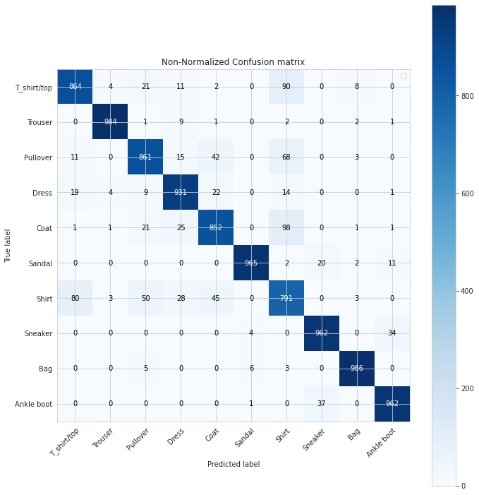

Similarly, we can visualize the same confusion matrix in a normalized form to see the percentage of correct and incorrect classifications by the model.

plt.figure(figsize = (20,20))
plot_confusion_matrix(y_test, predicted_classes, classes=class_names, normalize=True, title='Normalized Confusion matrix')
plt.axis('off')

As we can see in the above confusion matrix, our model has given the highest accuracy of 99% in recognizing bags, 98% in recognizing trousers and so on. The model has given the lowest accuracy of 79% in recognizing shirts. In recognizing apparels of more than 6 classes out of 10, it has given more than 90% accuracy and more than 85% accuracy in recognizing apparels of 9 classes. This level of accuracy in recognizing objects is definitely high. In further articles, we will check the same recognition accuracy by using different models.