


Clustering Example: 4 Steps You Should Know
This article describes k-means clustering example and provide a step-by-step guide summarizing the different steps to follow for conducting a cluster analysis on a real data set using R software.
We’ll use mainly two R packages:
- cluster: for cluster analyses and
- factoextra: for the visualization of the analysis results.
Install these packages, as follow:
install.packages(c("cluster", "factoextra"))A rigorous cluster analysis can be conducted in 3 steps mentioned below:
Here, we provide quick R scripts to perform all these steps.
Contents:
Related Book:
Data preparation
We’ll use the demo data set USArrests. We start by standardizing the data using the scale() function:
# Load the data set
data(USArrests)
# Standardize
df <- scale(USArrests)
Assessing the clusterability
The function get_clust_tendency() [factoextra package] can be used. It computes the Hopkins statistic and provides a visual approach.
library("factoextra")
res <- get_clust_tendency(df, 40, graph = TRUE)
# Hopskin statistic
res$hopkins_stat
## [1] 0.656# Visualize the dissimilarity matrix
print(res$plot)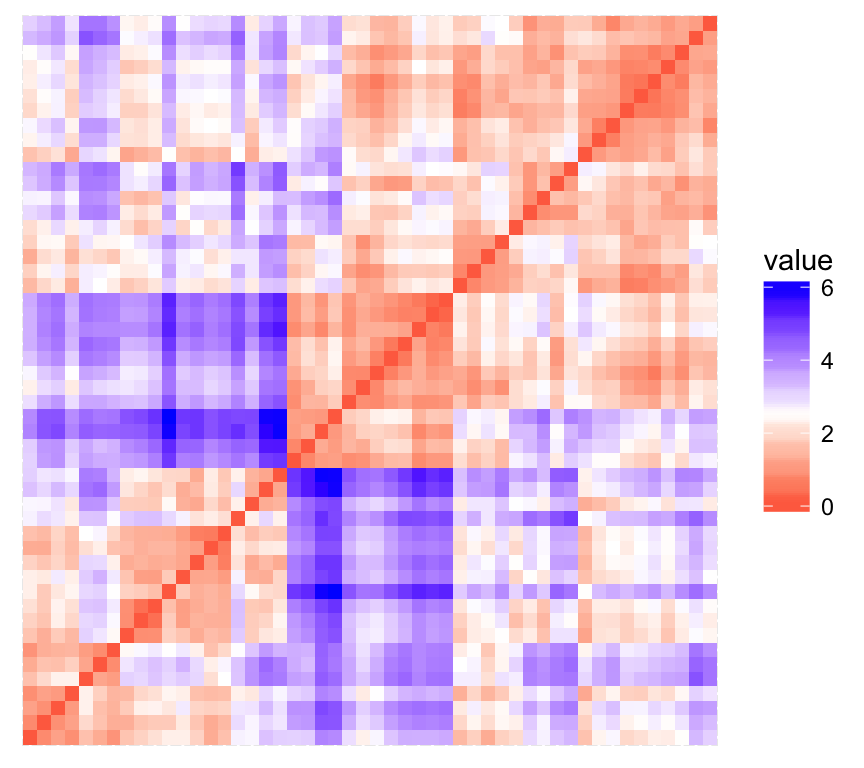
The value of the Hopkins statistic is significantly < 0.5, indicating that the data is highly clusterable. Additionally, It can be seen that the ordered dissimilarity image contains patterns (i.e., clusters).
Estimate the number of clusters in the data
As k-means clustering requires to specify the number of clusters to generate, we’ll use the function clusGap() [cluster package] to compute gap statistics for estimating the optimal number of clusters . The function fviz_gap_stat() [factoextra] is used to visualize the gap statistic plot.
library("cluster")
set.seed(123)
# Compute the gap statistic
gap_stat <- clusGap(df, FUN = kmeans, nstart = 25,
                    K.max = 10, B = 100)
# Plot the result
library(factoextra)
fviz_gap_stat(gap_stat)
The gap statistic suggests a 4 cluster solutions.
It’s also possible to use the function NbClust() [in NbClust] package.
It’s also possible to use the function NbClust() [NbClust package].
Compute k-means clustering
K-means clustering with k = 4:
# Compute k-means
set.seed(123)
km.res <- kmeans(df, 4, nstart = 25)
head(km.res$cluster, 20)
## Alabama Alaska Arizona Arkansas California Colorado
## 4 3 3 4 3 3
## Connecticut Delaware Florida Georgia Hawaii Idaho
## 2 2 3 4 2 1
## Illinois Indiana Iowa Kansas Kentucky Louisiana
## 3 2 1 2 1 4
## Maine Maryland
## 1 3# Visualize clusters using factoextra
fviz_cluster(km.res, USArrests)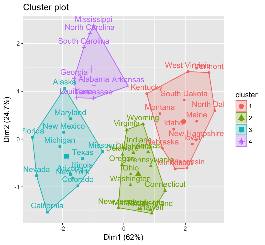
Cluster validation statistics: Inspect cluster silhouette plot
Recall that the silhouette measures (\(S_i\)) how similar an object \(i\) is to the the other objects in its own cluster versus those in the neighbor cluster. \(S_i\) values range from 1 to - 1:
- A value of \(S_i\) close to 1 indicates that the object is well clustered. In the other words, the object \(i\) is similar to the other objects in its group.
- A value of \(S_i\) close to -1 indicates that the object is poorly clustered, and that assignment to some other cluster would probably improve the overall results.
sil <- silhouette(km.res$cluster, dist(df))
rownames(sil) <- rownames(USArrests)
head(sil[, 1:3])
## cluster neighbor sil_width
## Alabama 4 3 0.4858
## Alaska 3 4 0.0583
## Arizona 3 2 0.4155
## Arkansas 4 2 0.1187
## California 3 2 0.4356
## Colorado 3 2 0.3265fviz_silhouette(sil)## cluster size ave.sil.width
## 1 1 13 0.37
## 2 2 16 0.34
## 3 3 13 0.27
## 4 4 8 0.39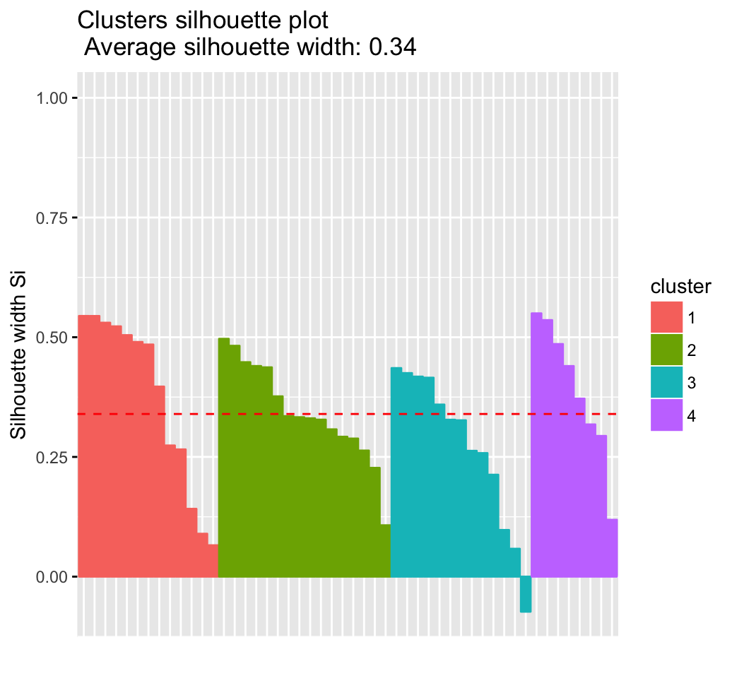
It can be seen that there are some samples which have negative silhouette values. Some natural questions are :
Which samples are these? To what cluster are they closer?
This can be determined from the output of the function silhouette() as follow:
neg_sil_index <- which(sil[, "sil_width"] < 0)
sil[neg_sil_index, , drop = FALSE]
## cluster neighbor sil_width
## Missouri 3 2 -0.0732eclust(): Enhanced clustering analysis
The function eclust()[factoextra package] provides several advantages compared to the standard packages used for clustering analysis:
- It simplifies the workflow of clustering analysis
- It can be used to compute hierarchical clustering and partitioning clustering in a single line function call
- The function eclust() computes automatically the gap statistic for estimating the right number of clusters.
- It automatically provides silhouette information
- It draws beautiful graphs using ggplot2
K-means clustering using eclust()
# Compute k-means
res.km <- eclust(df, "kmeans", nstart = 25)
# Gap statistic plot
fviz_gap_stat(res.km$gap_stat)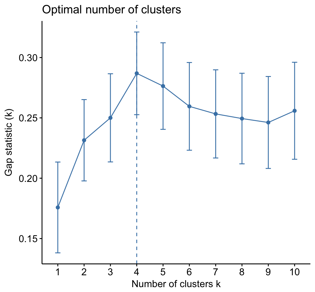
# Silhouette plot
fviz_silhouette(res.km)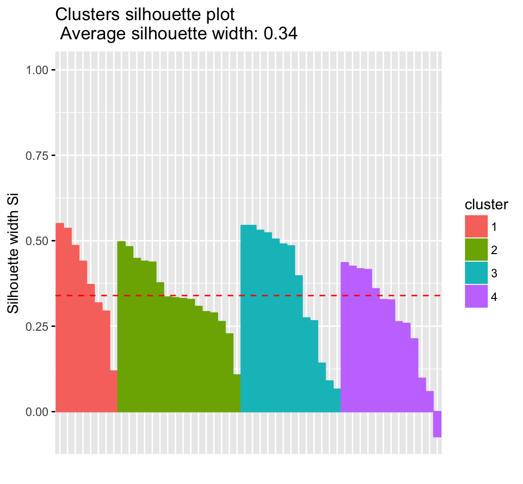
Hierachical clustering using eclust()
 # Enhanced hierarchical clustering
res.hc <- eclust(df, "hclust") # compute hclust
## Clustering k = 1,2,..., K.max (= 10): .. done
## Bootstrapping, b = 1,2,..., B (= 100) [one "." per sample]:
## .................................................. 50
## .................................................. 100fviz_dend(res.hc, rect = TRUE) # dendrogam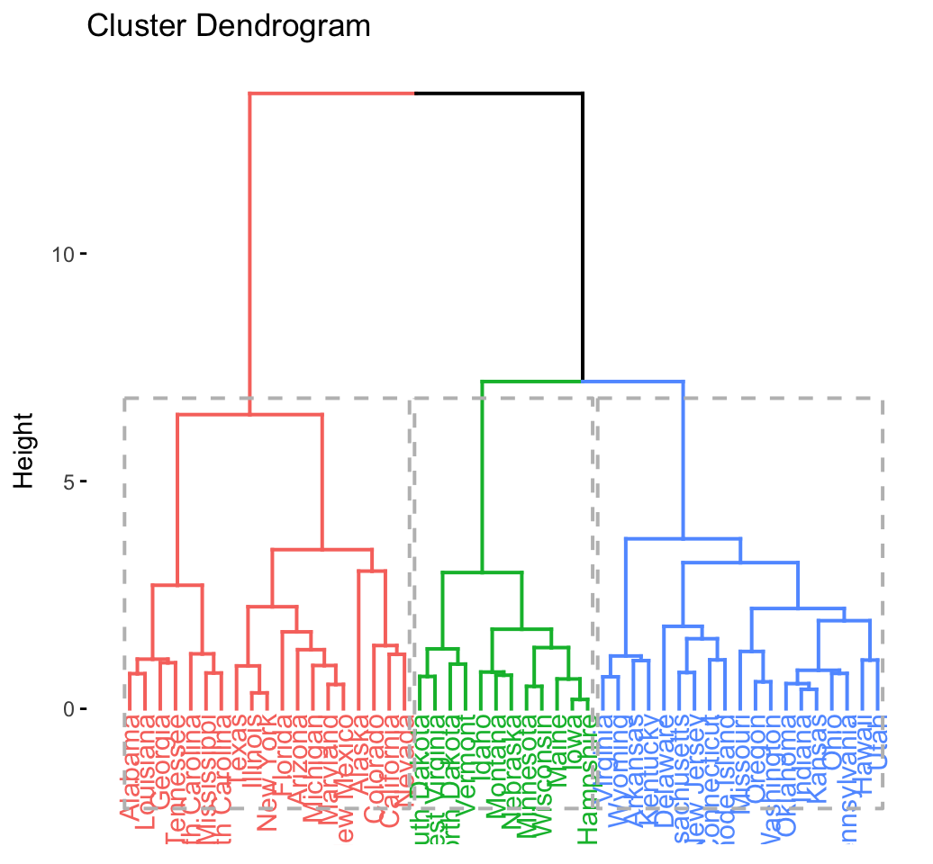
The R code below generates the silhouette plot and the scatter plot for hierarchical clustering.
fviz_silhouette(res.hc) # silhouette plot
fviz_cluster(res.hc) # scatter plot