


Cluster Analysis in R Simplified and Enhanced
In R, standard clustering methods (partitioning and hierarchical clustering) can be computed using the R packages stats and cluster. However the workflow, generally, requires multiple steps and multiple lines of R codes.
This article describes some easy-to-use wrapper functions, in the factoextra R package, for simplifying and improving cluster analysis in R. These functions include:
get_dist() & fviz_dist() for computing and visualizing distance matrix between rows of a data matrix. Compared to the standard dist() function, get_dist() supports correlation-based distance measures including “pearson”, “kendall” and “spearman” methods.
- eclust(): enhanced cluster analysis. It has several advantages:
- It simplifies the workflow of clustering analysis
- It can be used to compute hierarchical clustering and partititioning clustering in a single line function call
- Compared to the standard partitioning functions (kmeans, pam, clara and fanny) which requires the user to specify the optimal number of clusters, the function eclust() computes automatically the gap statistic for estimating the right number of clusters.
- For hierarchical clustering, correlation-based metric is allowed
- It provides silhouette information for all partitioning methods and hierarchical clustering
- It creates beautiful graphs using ggplot2
Required packages
We’ll use the factoextra package for an enhanced cluster analysis and visualization.
- Install factoextra:
install.packages("factoextra")- Load factoextra
library(factoextra)Data preparation
The built-in R dataset USArrests is used:
# Load and scale the dataset
data("USArrests")
df <- scale(USArrests)
head(df)
## Murder Assault UrbanPop Rape
## Alabama 1.2426 0.783 -0.521 -0.00342
## Alaska 0.5079 1.107 -1.212 2.48420
## Arizona 0.0716 1.479 0.999 1.04288
## Arkansas 0.2323 0.231 -1.074 -0.18492
## California 0.2783 1.263 1.759 2.06782
## Colorado 0.0257 0.399 0.861 1.86497Distance matrix computation and visualization
library(factoextra)
# Correlation-based distance method
res.dist <- get_dist(df, method = "pearson")
head(round(as.matrix(res.dist), 2))[, 1:6]
## Alabama Alaska Arizona Arkansas California Colorado
## Alabama 0.00 0.71 1.45 0.09 1.87 1.69
## Alaska 0.71 0.00 0.83 0.37 0.81 0.52
## Arizona 1.45 0.83 0.00 1.18 0.29 0.60
## Arkansas 0.09 0.37 1.18 0.00 1.59 1.37
## California 1.87 0.81 0.29 1.59 0.00 0.11
## Colorado 1.69 0.52 0.60 1.37 0.11 0.00# Visualize the dissimilarity matrix
fviz_dist(res.dist, lab_size = 8)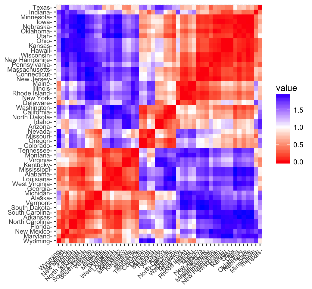
In the plot above, similar objects are close to one another. Red color corresponds to small distance and blue color indicates big distance between observation.
Enhanced clustering analysis
The standard R code for computing hierarchical clustering looks like this:
# Load and scale the dataset
data("USArrests")
df <- scale(USArrests)
# Compute dissimilarity matrix
res.dist <- dist(df, method = "euclidean")
# Compute hierarchical clustering
res.hc <- hclust(res.dist, method = "ward.D2")
# Visualize
plot(res.hc, cex = 0.5)
In this section we’ll describe the eclust() function [factoextra package] to simplify the workflow. The format is as follow:
eclust(x, FUNcluster = "kmeans", hc_metric = "euclidean", ...)- x: numeric vector, data matrix or data frame
- FUNcluster: a clustering function including “kmeans”, “pam”, “clara”, “fanny”, “hclust”, “agnes” and “diana”. Abbreviation is allowed.
- hc_metric: character string specifying the metric to be used for calculating dissimilarities between observations. Allowed values are those accepted by the function dist() [including “euclidean”, “manhattan”, “maximum”, “canberra”, “binary”, “minkowski”] and correlation based distance measures [“pearson”, “spearman” or “kendall”]. Used only when FUNcluster is a hierarchical clustering function such as one of “hclust”, “agnes” or “diana”.
- …: other arguments to be passed to FUNcluster.
In the following R code, we’ll show some examples for enhanced k-means clustering and hierarchical clustering. Note that the same analysis can be done for PAM, CLARA, FANNY, AGNES and DIANA.
library("factoextra")
# Enhanced k-means clustering
res.km <- eclust(df, "kmeans", nstart = 25)
## Clustering k = 1,2,..., K.max (= 10): .. done
## Bootstrapping, b = 1,2,..., B (= 100) [one "." per sample]:
## .................................................. 50
## .................................................. 100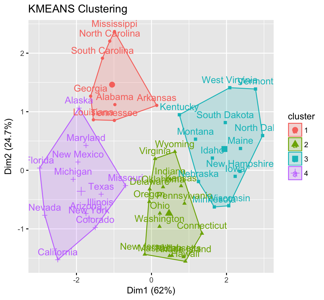
# Gap statistic plot
fviz_gap_stat(res.km$gap_stat)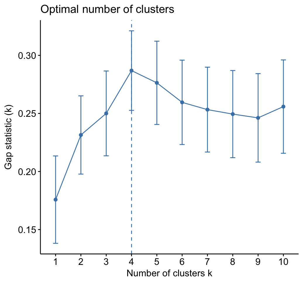
# Silhouette plot
fviz_silhouette(res.km)
## cluster size ave.sil.width
## 1 1 8 0.39
## 2 2 16 0.34
## 3 3 13 0.37
## 4 4 13 0.27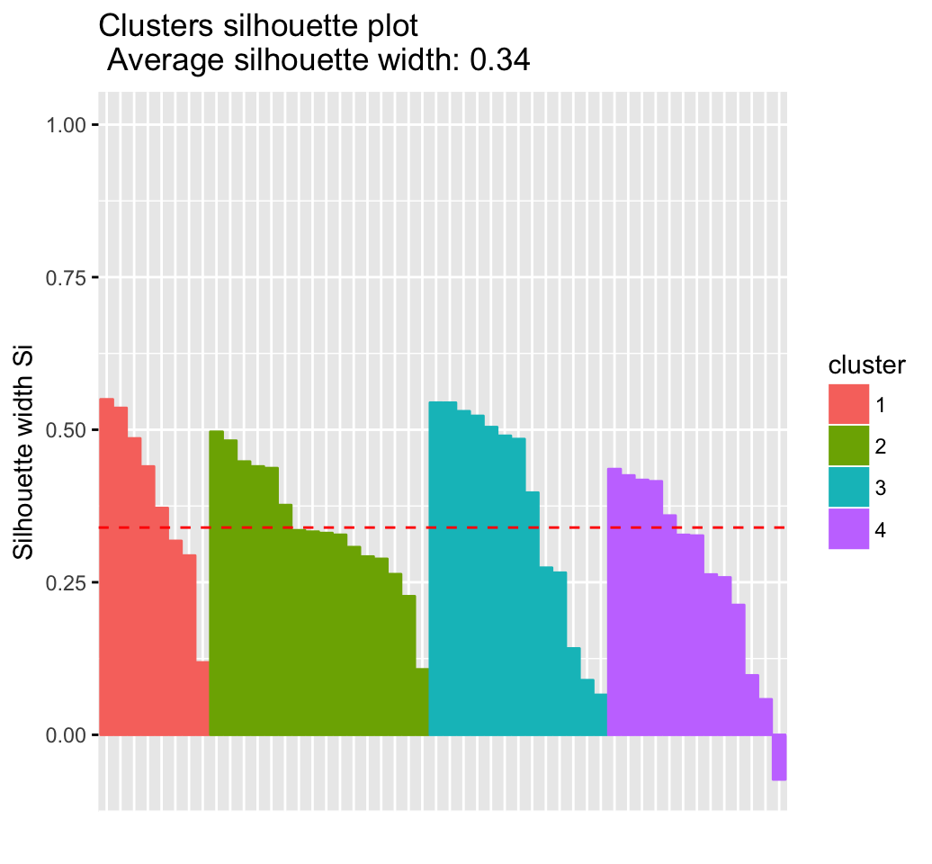
# Optimal number of clusters using gap statistics
res.km$nbclust
## [1] 4# Print result
res.km## K-means clustering with 4 clusters of sizes 8, 16, 13, 13
##
## Cluster means:
## Murder Assault UrbanPop Rape
## 1 1.412 0.874 -0.815 0.0193
## 2 -0.489 -0.383 0.576 -0.2617
## 3 -0.962 -1.107 -0.930 -0.9668
## 4 0.695 1.039 0.723 1.2769
##
## Clustering vector:
## Alabama Alaska Arizona Arkansas California
## 1 4 4 1 4
## Colorado Connecticut Delaware Florida Georgia
## 4 2 2 4 1
## Hawaii Idaho Illinois Indiana Iowa
## 2 3 4 2 3
## Kansas Kentucky Louisiana Maine Maryland
## 2 3 1 3 4
## Massachusetts Michigan Minnesota Mississippi Missouri
## 2 4 3 1 4
## Montana Nebraska Nevada New Hampshire New Jersey
## 3 3 4 3 2
## New Mexico New York North Carolina North Dakota Ohio
## 4 4 1 3 2
## Oklahoma Oregon Pennsylvania Rhode Island South Carolina
## 2 2 2 2 1
## South Dakota Tennessee Texas Utah Vermont
## 3 1 4 2 3
## Virginia Washington West Virginia Wisconsin Wyoming
## 2 2 3 3 2
##
## Within cluster sum of squares by cluster:
## [1] 8.32 16.21 11.95 19.92
## (between_SS / total_SS = 71.2 %)
##
## Available components:
##
## [1] "cluster" "centers" "totss" "withinss"
## [5] "tot.withinss" "betweenss" "size" "iter"
## [9] "ifault" "clust_plot" "silinfo" "nbclust"
## [13] "data" "gap_stat" # Enhanced hierarchical clustering
res.hc <- eclust(df, "hclust") # compute hclust## Clustering k = 1,2,..., K.max (= 10): .. done
## Bootstrapping, b = 1,2,..., B (= 100) [one "." per sample]:
## .................................................. 50
## .................................................. 100 fviz_dend(res.hc, rect = TRUE) # dendrogam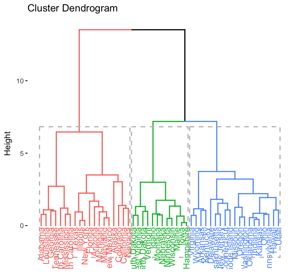
fviz_silhouette(res.hc) # silhouette plot## cluster size ave.sil.width
## 1 1 19 0.26
## 2 2 19 0.28
## 3 3 12 0.43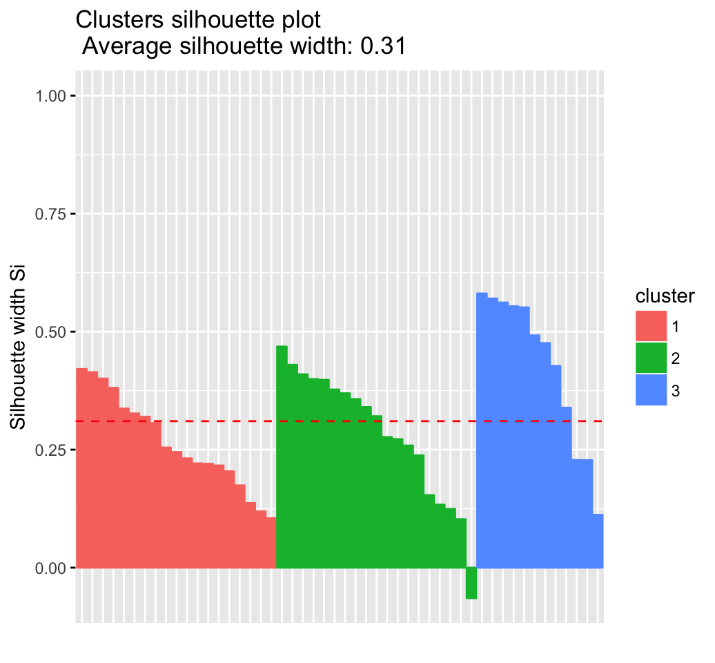
fviz_cluster(res.hc) # scatter plot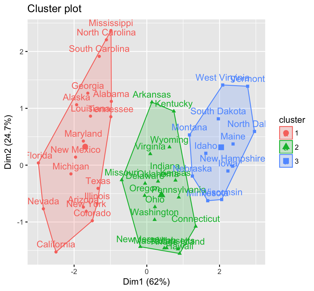
It’s also possible to specify the number of clusters as follow:
eclust(df, "kmeans", k = 4)