


DBSCAN: Density-Based Clustering Essentials
DBSCAN (Density-Based Spatial Clustering and Application with Noise), is a density-based clusering algorithm, introduced in Ester et al. 1996, which can be used to identify clusters of any shape in a data set containing noise and outliers.
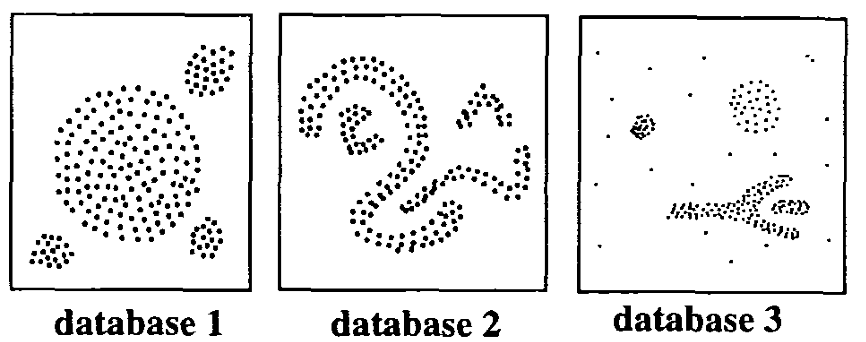
The basic idea behind the density-based clustering approach is derived from a human intuitive clustering method. For instance, by looking at the figure below, one can easily identify four clusters along with several points of noise, because of the differences in the density of points.
Clusters are dense regions in the data space, separated by regions of lower density of points. The DBSCAN algorithm is based on this intuitive notion of “clusters” and “noise”. The key idea is that for each point of a cluster, the neighborhood of a given radius has to contain at least a minimum number of points.
 (From Ester et al. 1996)
In this chapter, we’ll describe the DBSCAN algorithm and demonstrate how to compute DBSCAN using the fpc R package.
Contents:
Related Book:
Why DBSCAN?
Partitioning methods (K-means, PAM clustering) and hierarchical clustering are suitable for finding spherical-shaped clusters or convex clusters. In other words, they work well only for compact and well separated clusters. Moreover, they are also severely affected by the presence of noise and outliers in the data.
Unfortunately, real life data can contain: i) clusters of arbitrary shape such as those shown in the figure below (oval, linear and “S” shape clusters); ii) many outliers and noise.
The figure below shows a data set containing nonconvex clusters and outliers/noises. The simulated data set multishapes [in factoextra package] is used.
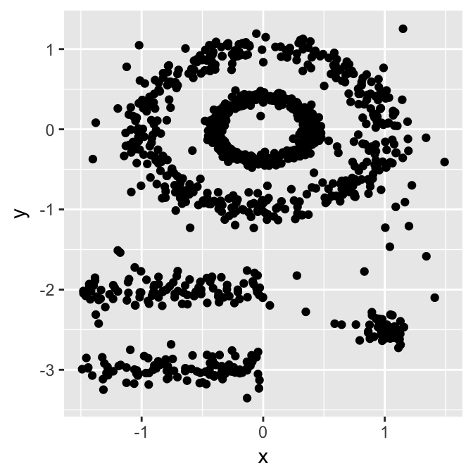
The plot above contains 5 clusters and outliers, including:
- 2 ovales clusters
- 2 linear clusters
- 1 compact cluster
Given such data, k-means algorithm has difficulties for identifying theses clusters with arbitrary shapes. To illustrate this situation, the following R code computes k-means algorithm on the multishapes data set. The function fviz_cluster()[factoextra package] is used to visualize the clusters.
First, install factoextra: install.packages(“factoextra”); then compute and visualize k-means clustering using the data set multishapes:
library(factoextra)
data("multishapes")
df <- multishapes[, 1:2]
set.seed(123)
km.res <- kmeans(df, 5, nstart = 25)
fviz_cluster(km.res, df,  geom = "point",
             ellipse= FALSE, show.clust.cent = FALSE,
             palette = "jco", ggtheme = theme_classic())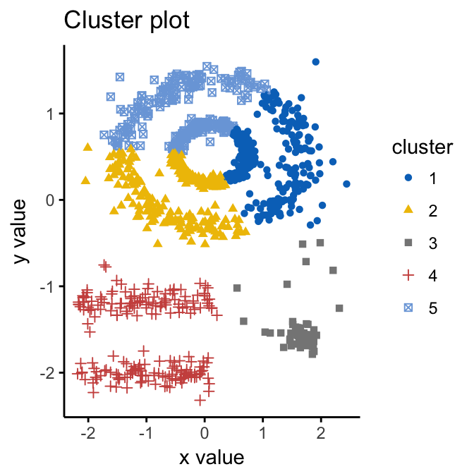
We know there are 5 five clusters in the data, but it can be seen that k-means method inaccurately identify the 5 clusters.
Algorithm
The goal is to identify dense regions, which can be measured by the number of objects close to a given point.
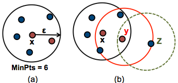
Two important parameters are required for DBSCAN: epsilon (“eps”) and minimum points (“MinPts”). The parameter eps defines the radius of neighborhood around a point x. It’s called called the \(\epsilon\)-neighborhood of x. The parameter MinPts is the minimum number of neighbors within “eps” radius.
Any point x in the data set, with a neighbor count greater than or equal to MinPts, is marked as a core point. We say that x is border point, if the number of its neighbors is less than MinPts, but it belongs to the \(\epsilon\)-neighborhood of some core point z. Finally, if a point is neither a core nor a border point, then it is called a noise point or an outlier.
The figure below shows the different types of points (core, border and outlier points) using MinPts = 6. Here x is a core point because \(neighbours_\epsilon(x) = 6\), y is a border point because \(neighbours_\epsilon(y) < MinPts\), but it belongs to the \(\epsilon\)-neighborhood of the core point x. Finally, z is a noise point.
We start by defining 3 terms, required for understanding the DBSCAN algorithm:
- Direct density reachable: A point “A” is directly density reachable from another point “B” if: i) “A” is in the \(\epsilon\)-neighborhood of “B” and ii) “B” is a core point.
- Density reachable: A point “A” is density reachable from “B” if there are a set of core points leading from “B” to “A.
- Density connected: Two points “A” and “B” are density connected if there are a core point “C”, such that both “A” and “B” are density reachable from “C”.
A density-based cluster is defined as a group of density connected points. The algorithm of density-based clustering (DBSCAN) works as follow:
-
For each point xi, compute the distance between xi and the other points. Finds all neighbor points within distance eps of the starting point (xi). Each point, with a neighbor count greater than or equal to MinPts, is marked as core point or visited.
-
For each core point, if it’s not already assigned to a cluster, create a new cluster. Find recursively all its density connected points and assign them to the same cluster as the core point.
-
Iterate through the remaining unvisited points in the data set.
Those points that do not belong to any cluster are treated as outliers or noise.
Advantages
- Unlike K-means, DBSCAN does not require the user to specify the number of clusters to be generated
- DBSCAN can find any shape of clusters. The cluster doesn’t have to be circular.
- DBSCAN can identify outliers
Parameter estimation
MinPts: The larger the data set, the larger the value of minPts should be chosen. minPts must be chosen at least 3.
\(\epsilon\): The value for \(\epsilon\) can then be chosen by using a k-distance graph, plotting the distance to the k = minPts nearest neighbor. Good values of \(\epsilon\) are where this plot shows a strong bend.
Computing DBSCAN
Here, we’ll use the R package fpc to compute DBSCAN. It’s also possible to use the package dbscan, which provides a faster re-implementation of DBSCAN algorithm compared to the fpc package.
We’ll also use the factoextra package for visualizing clusters.
First, install the packages as follow:
install.packages("fpc")
install.packages("dbscan")
install.packages("factoextra")
The R code below computes and visualizes DBSCAN using multishapes data set [factoextra R package]:
# Load the data
data("multishapes", package = "factoextra")
df <- multishapes[, 1:2]
# Compute DBSCAN using fpc package
library("fpc")
set.seed(123)
db <- fpc::dbscan(df, eps = 0.15, MinPts = 5)
# Plot DBSCAN results
library("factoextra")
fviz_cluster(db, data = df, stand = FALSE,
             ellipse = FALSE, show.clust.cent = FALSE,
             geom = "point",palette = "jco", ggtheme = theme_classic())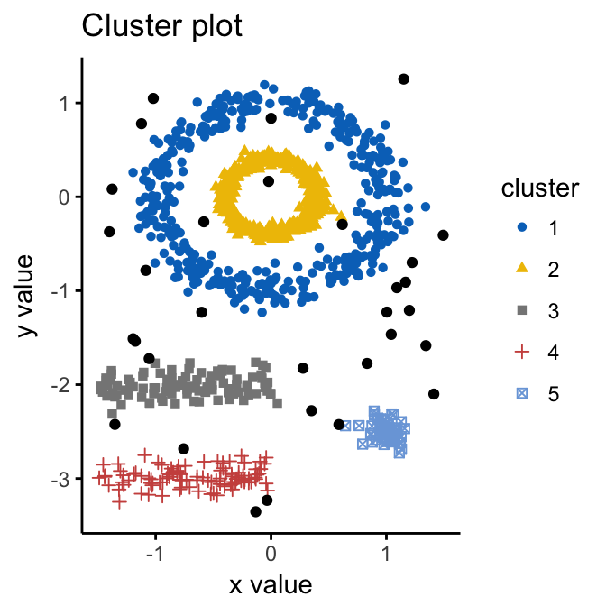
Note that, the function fviz_cluster() uses different point symbols for core points (i.e, seed points) and border points. Black points correspond to outliers. You can play with eps and MinPts for changing cluster configurations.
It can be seen that DBSCAN performs better for these data sets and can identify the correct set of clusters compared to k-means algorithms.
The result of the fpc::dbscan() function can be displayed as follow:
print(db)## dbscan Pts=1100 MinPts=5 eps=0.15
## 0 1 2 3 4 5
## border 31 24 1 5 7 1
## seed 0 386 404 99 92 50
## total 31 410 405 104 99 51In the table above, column names are cluster number. Cluster 0 corresponds to outliers (black points in the DBSCAN plot). The function print.dbscan() shows a statistic of the number of points belonging to the clusters that are seeds and border points.
# Cluster membership. Noise/outlier observations are coded as 0
# A random subset is shown
db$cluster[sample(1:1089, 20)]
## [1] 1 3 2 4 3 1 2 4 2 2 2 2 2 2 1 4 1 1 1 0DBSCAN algorithm requires users to specify the optimal eps values and the parameter MinPts. In the R code above, we used eps = 0.15 and MinPts = 5. One limitation of DBSCAN is that it is sensitive to the choice of \(\epsilon\), in particular if clusters have different densities. If \(\epsilon\) is too small, sparser clusters will be defined as noise. If \(\epsilon\) is too large, denser clusters may be merged together. This implies that, if there are clusters with different local densities, then a single \(\epsilon\) value may not suffice.
A natural question is:
How to define the optimal value of ?
Method for determining the optimal eps value
The method proposed here consists of computing the k-nearest neighbor distances in a matrix of points.
The idea is to calculate, the average of the distances of every point to its k nearest neighbors. The value of k will be specified by the user and corresponds to MinPts.
Next, these k-distances are plotted in an ascending order. The aim is to determine the “knee”, which corresponds to the optimal eps parameter.
A knee corresponds to a threshold where a sharp change occurs along the k-distance curve.
The function kNNdistplot() [in dbscan package] can be used to draw the k-distance plot:
dbscan::kNNdistplot(df, k =  5)
abline(h = 0.15, lty = 2)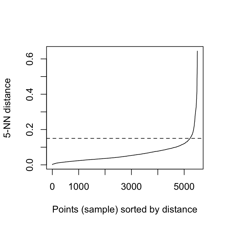
It can be seen that the optimal eps value is around a distance of 0.15.
Cluster predictions with DBSCAN algorithm
The function predict.dbscan(object, data, newdata) [in fpc package] can be used to predict the clusters for the points in newdata. For more details, read the documentation (?predict.dbscan).