
DANNP: an efficient artificial neural network pruning tool
- Published
- Accepted
- Received
- Academic Editor
- Sebastian Ventura
- Subject Areas
- Algorithms and Analysis of Algorithms, Artificial Intelligence, Data Mining and Machine Learning
- Keywords
- Artificial neural networks, Pruning, Parallelization, Feature selection, Classification problems, Machine learning, Artificial inteligence
- Copyright
- © 2017 Alshahrani et al.
- Licence
- This is an open access article distributed under the terms of the Creative Commons Attribution License, which permits unrestricted use, distribution, reproduction and adaptation in any medium and for any purpose provided that it is properly attributed. For attribution, the original author(s), title, publication source (PeerJ Computer Science) and either DOI or URL of the article must be cited.
- Cite this article
- 2017. DANNP: an efficient artificial neural network pruning tool. PeerJ Computer Science 3:e137 https://doi.org/10.7717/peerj-cs.137
Abstract
Background
Artificial neural networks (ANNs) are a robust class of machine learning models and are a frequent choice for solving classification problems. However, determining the structure of the ANNs is not trivial as a large number of weights (connection links) may lead to overfitting the training data. Although several ANN pruning algorithms have been proposed for the simplification of ANNs, these algorithms are not able to efficiently cope with intricate ANN structures required for complex classification problems.
Methods
We developed DANNP, a web-based tool, that implements parallelized versions of several ANN pruning algorithms. The DANNP tool uses a modified version of the Fast Compressed Neural Network software implemented in C++ to considerably enhance the running time of the ANN pruning algorithms we implemented. In addition to the performance evaluation of the pruned ANNs, we systematically compared the set of features that remained in the pruned ANN with those obtained by different state-of-the-art feature selection (FS) methods.
Results
Although the ANN pruning algorithms are not entirely parallelizable, DANNP was able to speed up the ANN pruning up to eight times on a 32-core machine, compared to the serial implementations. To assess the impact of the ANN pruning by DANNP tool, we used 16 datasets from different domains. In eight out of the 16 datasets, DANNP significantly reduced the number of weights by 70%–99%, while maintaining a competitive or better model performance compared to the unpruned ANN. Finally, we used a naïve Bayes classifier derived with the features selected as a byproduct of the ANN pruning and demonstrated that its accuracy is comparable to those obtained by the classifiers trained with the features selected by several state-of-the-art FS methods. The FS ranking methodology proposed in this study allows the users to identify the most discriminant features of the problem at hand. To the best of our knowledge, DANNP (publicly available at www.cbrc.kaust.edu.sa/dannp) is the only available and on-line accessible tool that provides multiple parallelized ANN pruning options. Datasets and DANNP code can be obtained at www.cbrc.kaust.edu.sa/dannp/data.php and https://doi.org/10.5281/zenodo.1001086.
Introduction
Artificial neural networks (ANNs) can arbitrarily well approximate non-linear target functions (Bishop, 2006). An extensive empirical study (Fernandez-Delgado, Cernadas & Barro, 2014) demonstrated that a voting ensemble of ANNs achieved the best average performance over the UCI machine learning repository on two-class classification problems. The ANNs have been extensively used for solving different classification problems, see, for example, (Almeida, 2002; Ashoor et al., 2011; Bajic et al., 2002; Bajic et al., 2004; Bajic & Werner, 2005; Basheer & Hajmeer, 2000; Dias, Antunes & Mota, 2004; Gan, Chen & Huang, 2016; Gardnera & Dorlinga, 1998; Hatzigeorgiou, 2002; Hernández-Serna & Jiménez-Segura, 2014; Jayne, Iliadis & Mladenov, 2016; Kalkatawi et al., 2013; Li et al., 2015; Magana-Mora et al., 2013; Magana-Mora & Bajic, 2017; Magana-Mora, Kalkatawi & Bajic, 2017; Meireles, Almeida & Simoes, 2003; Wang et al., 2017). The ANNs are universal approximators, given a sufficiently rich model architecture and weights (Hornik, Stinchcombe & White, 1989), and may consist of multiple hidden layers. However, the multilayer ANN representation rapidly increases model complexity due to the large number of tunable weights. Moreover, the high number of weights may amplify irrelevant characteristics or noise that may be present in the training data and lead to a poor model generalization for unseen data. This problem is referred to as overfitting of the training data, and different methods have been proposed to address this undesirable effect. These methods may be broadly divided into three groups: (1) ANN regularization (Ng, 2004; Nowlan & Hinton, 1992), (2) early stopping (Prechelt, 2012), and (3) ANN pruning (Burden & Winkler, 2009; Reed, 1993; Srivastava et al., 2014; Wan et al., 2013). Here, we focus on the ANN pruning as it not only simplifies the model structure but also results in fewer computations and smaller storage requirements for the pruned network. In addition, as a side benefit, the ANN pruning may keep the most useful features and rank their relevance based on their predictive capabilities. Although there are different robust methods for performing feature selection (FS) and feature ranking, selection of the FS method and the parameters is not trivial. Refer to Soufan et al. (2015b) for more details on FS.
ANN pruning algorithms may be divided into two categories. The simplest, magnitude-based pruning (MP) methods consist of removing weights with the lowest magnitudes. After a certain number of weights are deleted, the ANN is retrained. While this approach may work for some problems, removing weights with the smallest magnitudes does not always produce the smallest increase of the error function (Hassibi, Stork & Wolff, 1993). More sophisticated, the second category of pruning algorithms measures the sensitivity of the second-order information of the error function with respect to the weights. As a result, the weight that least increases the error function is removed (Hassibi, Stork & Wolff, 1993; Karnin, 1990; Mozer & Smolensky, 1989). These approaches usually result in more accurate models as they take advantage of the Hessian matrix (referred to as H matrix, hereafter) to account for the additional curvature information of the error function (Hassibi, Stork & Wolff, 1993). In this category of pruning algorithms, optimal brain damage (OBD) (LeCun et al., 1989) uses the second-order derivative of the error function relative to the network weights. The OBD avoids the complexity of computing the H matrix by assuming diagonal H-matrix. Nevertheless, this assumption is not true in many cases leading to the removal of the wrong weights (Hassibi, Stork & Wolff, 1993), and therefore, affects the accuracy of the resulting models. In contrast to OBD, the optimal brain surgeon (OBS) algorithm (Hassibi, Stork & Wolff, 1993) does not assume a diagonal H matrix. Additionally, OBS provides an approximation of the inverse H matrix (H- inverse) and is shown to produce more robust models than MP and OBD algorithms (Hassibi, Stork & Wolff, 1993). Refer to Article S1 for further details about these methods.
However, the pruning of ANNs is a computationally expensive task that often limits its application to real-life problems where datasets may contain a large number of samples and data features. Therefore, speeding up the pruning process is essential for many practical applications. Although pruning algorithms of the OBS types are not entirely parallelizable, certain computationally intensive parts are, which lead to a significant speedup on multicore processors. For the reasons mentioned above, this study aims to develop a user-friendly tool with several implemented parallelized ANN pruning algorithms able to cope with complex or medium size data. For this, we developed DANNP tool, which implements several parallelized variants of ANN pruning algorithms. We demonstrated the efficiency and utility of the implemented algorithms in the DANNP tool on several small to medium size benchmark datasets. Moreover, as a useful by-product of the ANN pruning, the pruning process selects the most useful data features for the problem in hand. The application of the FS methods to find a subset of features to train a classification model is often used to derive simpler and faster models. Although in many cases the reduced number of features may result in improved performance, the feature subset is not always capable of describing the data accurately and may frequently result in models with inferior performance. In this study, we demonstrate that the selected features result in similar or improved classification performance in comparison with several state-of-the-art FS methods on the considered datasets.
Materials and Methods
In this section, we first define the Hessian-based pruning algorithm and the implemented modifications for the parallelization of the code, followed by the details on the FS methods. Finally, we describe the datasets and model evaluation procedure to assess the performance of the DANNP tool.
Hessian-based pruning formulation and DANNP parallelization
The OBS uses the second-order information of the error function and measures the saliency of the ANN weights. The algorithm evaluates the saliency by the effect on the error function when the ANN weight vector w is perturbed. Therefore, the algorithm aims to determine the weights that cause the least increase of the error function E. The error function may be approximated by a Taylor series as follows (Hassibi, Stork & Wolff, 1993):
(1)
where E′(w) is the first-order derivative of E with respect to w (the gradients vector); H is the H matrix determined as H = ∂2E∕∂w2, i.e., as the second-order derivative of E with respect to w. The approximation of the H-inverse is obtained via an iterative procedure as follows (Hassibi, Stork & Wolff, 1993): (2)
where , I is the identity matrix and α is a small scalar; is the gradient vector from the backpropagation calculations in iteration m + 1, where m denotes the number of iterations; p is a scalar that represents the number of training samples. The H matrix is of size v2, where v is the total number of weights in the network.
The code optimization and parallelization of the pruning methods implemented in the DANNP tool are achieved by (1) implementation of a faster version of the algorithm for the approximation of the H-inverse, and (2) reducing the number of evaluations of the H-inverse approximation. To address the faster algorithm for approximation of the H-inverse, we modified the implementation of the calculation of the H-inverse using, where applicable, optimized BLAS routines (Blackford et al., 2002) and modified the code to reduce the overhead by computing repeated terms only once. However, since the approximation of the H-inverse is based on an iterative process (Eq. (2)), this inherent limitation hinders full parallel scaling. Algorithm 1 describes the implementation of the parallel version of Eq. (2) based on the BLAS routines. To address the reduction of the number of evaluations of the H-inverse approximation, we implemented multiple-weights OBS (MWOBS-parallel), which removes multiple weights in each pruning iteration while using the optimization described in Algorithm 1. In contrast to OBS where the H-inverse has to be computed for removing a single weight, in MWOBS-parallel this computation is performed only once for removing n weights, where the number of n weights is set to 1% of the weights in the initial ANN. This approach significantly reduces the running time and frequently achieves comparable or better performance relative to the serial OBS or the fully connected ANNs.
ANN model
The ANN models were derived by using a modified version of the Fast Compressed Neural Network software (Klima, 2015). This software is a modular and fast C++ implementation of ANN algorithms. We modified the software to use optimized BLAS to replace the serial approximation of the H-inverse update routines (using Eq. (2)).
In this study, we considered ANN with a single layer as it has been demonstrated that one hidden layer, with a sufficient number of nodes and a sigmoid activation function, is enough to learn complex data patterns (Cybenko, 1989; Hornik, Stinchcombe & White, 1989). However, our solutions apply to multilayer ANN architecture. Moreover, the resilient backpropagation algorithm (Riedmiller, 1994) was used to train the ANN as it frequently achieves faster convergence over the conventional backpropagation algorithm. Finally, we considered a different number of nodes in the hidden layer for comparing the pruning effects of different algorithms. The total number of weights correlates with the ANN complexity and is calculated as follows: (3)
where NumInputs, NumHNodes, and NumClasses refer to the number of input features, the number of nodes in the hidden layer, and the number of classes in the classification problem, respectively.
ANN pruning solutions implemented in DANNP tool
The DANNP tool implements the parallel versions of three OBS-based approaches to ANN pruning using the approximation of the H-inverse. These generate simpler structures and improve the model generalization with the least sacrifice in accuracy, compared to MP and OBD. The implemented algorithms are OBS-parallel, MWOBS-parallel, and unit-based OBS (UOBS-parallel), which are described in the following subsections. However, we also provide the simple MP algorithm for the sake of comparison. We did not compare against OBD algorithm as it has been shown that assuming a diagonal H matrix leads to the removal of wrong weights and produces inferior models (Hassibi, Stork & Wolff, 1993). In our implementation, pruning algorithms continue to remove weights as long as the increase in the training mean-squared error (MSE) is below 1% or stops when it reaches the pre-specified number of iterations.
OBS-parallel
The OBS algorithm aims to find the weight that when eliminated, it causes overall the least increase in the error function ΔEi calculated according to (4)
where wi refers to the i-th weight that is to be removed.
In this algorithm, the calculation of the H-inverse is required to remove a single weight per pruning iteration (Fig. 1A). Finally, the remaining weights in the network are updated to account for the removed weight (see Article S1 for further details).
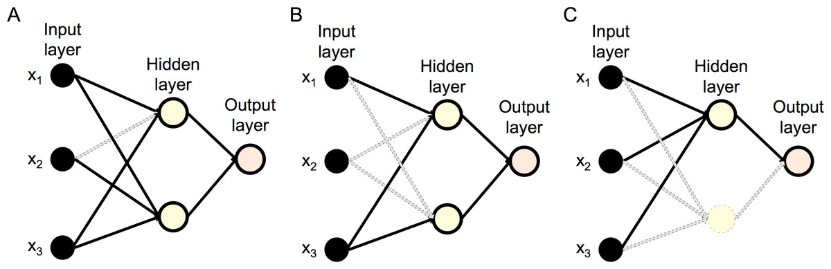
Figure 1: Pruning variants of OBS.
(A) OBS algorithm: a single weight (dashed line) is removed per pruning iteration. (B) MWOBS algorithm: multiple weights (dashed lines) are removed per pruning iteration. (C) UOBS algorithm: a node and its incoming/outgoing weights are removed in a pruning iteration.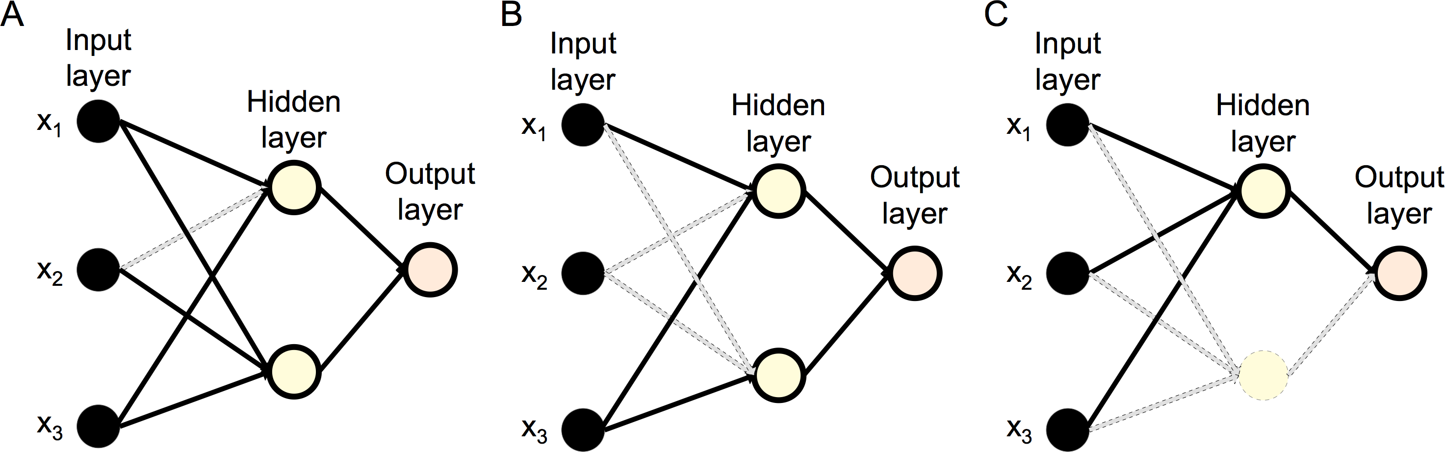
MWOBS-parallel
In contrast to OBS, the MWOBS algorithm may remove multiple weights in a single pruning iteration (Fig. 1B). To achieve this, the error increase ΔEi is evaluated individually for every weight in the network by using Eq. (4). Weights are then sorted according to the increase of the associated errors and the n weights with the smallest error increase are selected for pruning, where n is set to 1% of the weighs in the initial ANN. This simplification is made to avoid evaluating every combination of weights as described in the general formulation of pruning n weights using OBS in Stahlberger & Riedmiller (1997).
UOBS-parallel
The UOBS variant described in Stahlberger & Riedmiller (1997) defines a heuristic that leads to removal of all outgoing weights of a particular node, thus reducing the overall number of considered nodes in the network (Fig. 1C). We implemented this variant for the purpose of completeness, and integrated the optimized parallel approximation of the H-inverse in this approach, as indicated in Algorithm 1.
Feature selection through ANN pruning and comparison settings
Due to the simplification of the ANN structure through pruning, it is possible that some of the input data features are not used in the pruned ANN. This amounts to the FS in the wrapper setting. Figure 1B shows an example of a pruned ANN where input feature x2 is discarded (having no connecting weights from the input to the hidden layer). We ranked, in descending order, the remaining features (x1 and x3, from the example) by considering, for each input feature, the sum of the absolute values of all outgoing weights.
Similar to the comprehensive analysis of FS methods performed in Soufan et al. (2015b), we analyzed the pruning effects of the MWOBS-parallel variant on the features and compared it with the state-of-the-art methods for FS. We considered seven different FS methods from the FEAST MATLAB toolbox (Brown et al., 2012), namely, conditional mutual information maximization (CMIM) (Fleuret, 2004), correlation-based FS (Hall, 1999), joint mutual information (JMI) (Yang & Moody, 1999), maximum relevance minimum redundancy (mRMR) (Peng, Long & Ding, 2005), RELIEF (Kira & Rendell, 1992), T-test (Guyon & Elisseeff, 2003), and receiver operating characteristic curve (ROC) (Guyon & Elisseeff, 2003). Refer to Article S2 for more details on the FS methods.
We used MWOBS-parallel for determining the feature subsets, as it can cope with complex datasets and ANN structures requiring short running times. Since the selected features are the result of the ANN pruning, using an ANN to assess the performance of the feature subset may produce biased results. Thus, we used a naïve Bayes classifier to produce unbiased results with the so selected features.
Datasets
We measured the performance of the implemented ANN pruning algorithms, on 15 datasets from different domains and one synthetic dataset, all with a different number of features and number of samples. The selected datasets reflect some of the data properties present in real applications, i.e., small or medium size datasets represented by both small and large number of features. From these datasets, seven are taken from the UCI machine learning repository (Lichman, 2013), and nine are obtained from recent studies (Anguita et al., 2013; Johnson & Xie, 2013; Schmeier, Jankovic & Bajic, 2011; Singh et al., 2002; Soufan et al., 2015a; Tsanas et al., 2014; Wang et al., 2016; Yeh & Lien, 2009). Table 1 shows the summary information for these datasets.
| Datasets | Number of features | Number of samples | Number of classes |
|---|---|---|---|
| Breast cancer (BC) | 9 | 682 | 2 |
| Heart disease (HD) | 13 | 297 | 2 |
| Wisconsin diag. breast cancer (WDBC) | 30 | 569 | 2 |
| Promoters prediction (PP) | 57 | 106 | 2 |
| Cardiac arrhythmia (CA) | 277 | 442 | 2 |
| Synthetic madelon (SM) | 500 | 2,000 | 2 |
| Prostate cancer (PC) | 2,135 | 102 | 2 |
| TF-TF combination (TFTF) | 1,062 | 674 | 2 |
| AID886 compounds (AID) | 918 | 10,471 | 2 |
| Default credit cards (DCC) | 24 | 12,000 | 2 |
| Epileptic seizure recognition (ESR) | 178 | 11,500 | 2 |
| LSVT voice rehabilitation (LSVT) | 310 | 127 | 2 |
| Urban land cover (ULC) | 147 | 168 | 9 |
| Sensorless drive diagnosis (SDD) | 48 | 48,487 | 11 |
| Human activity recognition (HAR) | 561 | 10,299 | 6 |
| MNIST digits (MD) | 748 | 59,999 | 10 |
Data processing and model evaluation
Feature values for all considered datasets were normalized to have values within the range of [−1, 1]. We used the k-fold cross-validation technique to estimate the performance of ANNs. k-fold cross-validation requires dividing the whole dataset into k subsets of similar size. We train the ANN model on k − 1 subsets and test it on the remaining subset. The procedure repeats for each of the subsets and performance achieved is given as the average across all subsets. In this study, we used k = 10.
We used several statistical measures to evaluate the k-fold cross-validation performance. These metrics are accuracy, sensitivity, specificity, geometric mean (GM), and mean squared error (MSE). Table 2 defines the considered statistical performance metrics. In addition to these measures, Table S2 shows the results using Cohen’s kappa coefficient, recall, precision and F1 score. To evaluate the utility of the features obtained from the ANN pruning, we compared the accuracy of a naïve Bayes classifier generated with these selected features to the accuracy of naïve Bayes classifiers generated with features selected by seven other FS methods.
| Statistical measure | Equation |
|---|---|
| Accuracy | |
| Sensitivity | |
| Specificity | |
| GM | |
| MSE |
Results and Discussion
Here, we discuss in more details the speedup results obtained by the optimized parallel OBS variants, the accuracy resulting from ANN pruning and the effects on input features and weights. Finally, we present and discuss the results of the comprehensive comparisons for several state-of-the-art methods for FS, with FS and ranking based on ANN pruning. Three variants of the OBS pruning method using code parallelization are implemented in DANNP: (1) OBS-parallel, which eliminates only one weight per iteration; (2) MWOBS-parallel, which is an OBS variant that eliminates multiple weights per pruning iteration; and (3) unit-based OBS (UOBS-parallel), which eliminates a whole node (unit) and their connecting weights per iteration. For the sake of comparison, we also include the simple MP method.
Running time speedup
The speedup metric was used to quantify the running time reduction that we were able to achieve by parallelizing the calculation of the approximation of the H-inverse. The speedup is measured as follows: (5)
The performance gain obtained by parallelization is dictated by Amdahl’s law, which states that the optimization of the code is limited by the execution time of the code that cannot be parallelized (Amdahl, 1967). Specifically, for ANNs pruning, the most computationally demanding portion of the program is the calculation of the H-inverse. Therefore, we optimized the approximation of the H-inverse as described in Algorithm 1. Although MWOBS-parallel was able to cope with the datasets that are described by a relatively large number of samples and input features (i.e., CA, SM, PC, TFTF, AID, ESR, LSVT, ULC, HAR, DCC, SDD, and MD), the serial implementation of the OBS was not able to produce an output in an acceptable amount of time (<48 h). Therefore, Figs. 2A–2D show the speedup improvements of OBS-parallel and MWOBS-parallel over the non-parallel OBS in four datasets (BC, HD, WDCB, and PP). Table S1 shows the running time for the OBS-parallel, MWOBS-parallel, and UOBS-parallel for the remaining 12 datasets in which the OBS was unable to complete the execution within 48 h.
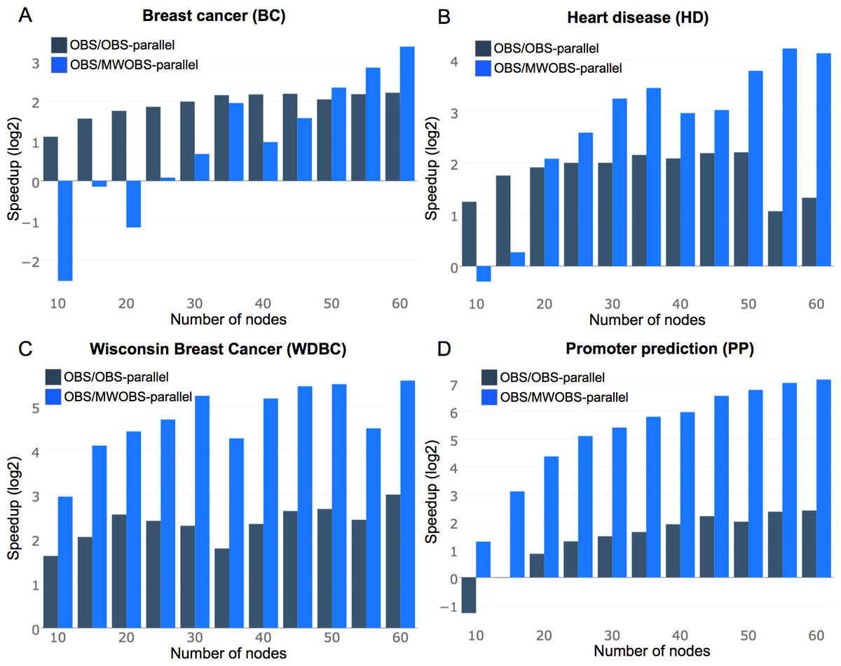
Figure 2: Speedup comparisons of OBS against OBS-parallel and MWOBS-parallel.
(A–D) Speedup comparison for datasets where the OBS algorithm was completed within 48 h. The y-axis shows the log2 of the speedup calculated from Eq. (5). The x-axis shows the number of nodes in the ANN.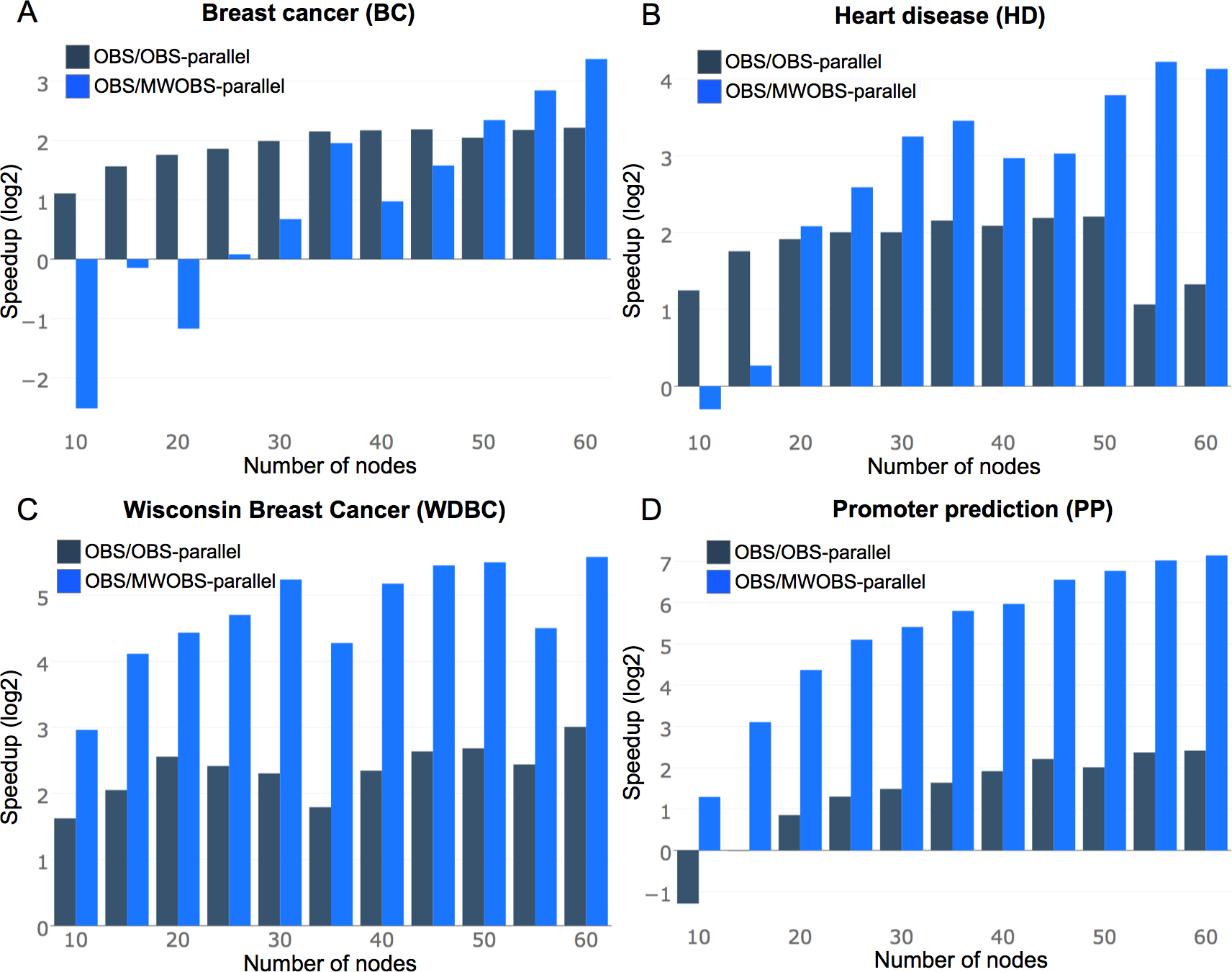
Results in Fig. 2 and Table S1 show that OBS-parallel consistently reduced the running time compared to the standard OBS in the 16 considered datasets. The MWOBS-parallel achieved slower running times in the BC dataset with a small number of nodes in the hidden layer. This may be due to the possible time required to rank the weights based on the error increase (see the Methods section). However, this overhead is marginal and may be ignored when increasing the number of weights in the ANN (by increasing the number of nodes in the hidden layer or for datasets with more input features). The significant enhancements in the running time are noticeable for WDBC and PP datasets containing samples described by 30 and 57 input features, respectively. For instance, in an ANN model with 60 nodes in the hidden layer for PP dataset (containing 3,540 weights, from Eq. (3)), the OBS-parallel algorithm runs ∼5.3 times faster than the serial OBS implementation. The main advantage of MWOBS-parallel algorithms is that it requires fewer evaluations of the H-inverse and when coupled with a parallel approximation of the H-inverse, more speedup is achieved.
Furthermore, we compared the performance of the pruning variants implemented in DANNP against the OBS implementation in NNSYSID MATLAB toolbox (Norgaard, Ravn & Poulsen, 2002). The NNSYSID is a toolbox for the identification of nonlinear dynamic systems with ANNs, often used as a benchmark, which implements several algorithms for ANN training and pruning. The fair comparison between the DANNP and NNSYSID tools is not possible since NNSYSID runs under MATLAB R2017b environment. Still, to get an insight about how much time is needed for the same tasks with these two tools, the NNSYSID and the pruning variants implemented in DANNP were run under the same conditions. These include the same data partitioning, activation functions, hidden units, training algorithms, and tolerance level. Data were partitioned into 15% testing, 15% validation, and 70% training. Table 3 shows the execution time comparison between DANNP and NNSYSID toolbox. For datasets with more features and samples, NNSYSID fails to scale for datasets with a larger number of features. These results show the running time improvement obtained by our implementation to approximate the H-inverse.
| Dataset | OBS-parallel | MWOBS-parallel | UOBS-parallel | MP | NNSYSID | No. of weights |
|---|---|---|---|---|---|---|
| BC | 0.0015 | 0.0014 | 0.0015 | 0.0008 | 0.509 | 111 |
| HD | 0.0024 | 0.0022 | 0.0011 | 0.0006 | 0.532 | 151 |
| WDBC | 0.0041 | 0.0025 | 0.0049 | 0.0014 | 4.682 | 321 |
| PP | 0.0130 | 0.0084 | 0.0454 | 0.0001 | 4.256 | 591 |
| CA | 0.3186 | 0.2632 | 3.1448 | 0.0049 | >24 h | 2,791 |
| SM | 6.3967 | 2.1337 | 69.5910 | 0.0332 | >24 h | 5,021 |
| PC | 763.596 | 424.894 | >24 h | 0.0181 | >24 h | 21,371 |
| TFTF | 25.6599 | 12.5185 | 213.0404 | 0.0174 | >24 h | 10,641 |
| AID | 17.6707 | 11.6155 | 61.1201 | 0.3885 | >24 h | 9,201 |
| ULC | 0.7904 | 0.1643 | 2.1006 | 0.0015 | 91.583 | 1,579 |
| SDD | 3.8972 | 1.5572 | 1.7080 | 0.2247 | >24 h | 611 |
| MD | 98.4303 | 10.9182 | 179.1087 | 2.1471 | >24 h | 7,960 |
| HAR | 44.4636 | 5.0967 | 312.4713 | 0.2015 | >24 h | 5,686 |
| ESR | 1.4119 | 0.5829 | 0.5537 | 0.0871 | >24 h | 1,801 |
| LSVT | 1.7044 | 0.7471 | 6.2507 | 0.0004 | >24 h | 3,121 |
| DCC | 0.1215 | 0.1185 | 0.0476 | 0.0238 | 90.161 | 261 |
So far, we have only analyzed the running time of the implemented ANN pruning algorithms. Next, we discuss in details the effects of the pruning algorithms in the ANN training error, cross-validation performance and on the FS resulting from the pruning.
Effects of different pruning algorithms on the ANN training error
Apart from the running time, the main difference in the ANN pruning algorithms is the selection of the weights to be removed during a pruning iteration. To investigate the effects of the different ANN pruning algorithms on the network, we evaluated the training performance through pruning steps until all weights are removed. The aim is to derive the simplest ANN structure (smaller number of weights) without increasing the MSE on the training data. Figures 3A–3J and Fig. S1 show the effects of the different pruning algorithms on the MSE. From these results, we observed that different pruning algorithms (including MP) were able to retain very few network weights without increasing the MSE for some datasets (i.e., PC and PP). However, the MP algorithm produced the highest MSE compared to the other algorithms for the remaining datasets. This is because the MP algorithm does not account for the effects of the removed weights on the network error (as mentioned in the ‘Introduction’) and thus, tends to remove the incorrect weights, which may significantly increase the error. Conversely, MWOBS-parallel consistently achieved the minimum increase in the MSE compared to the other pruning algorithms in all of the considered datasets.
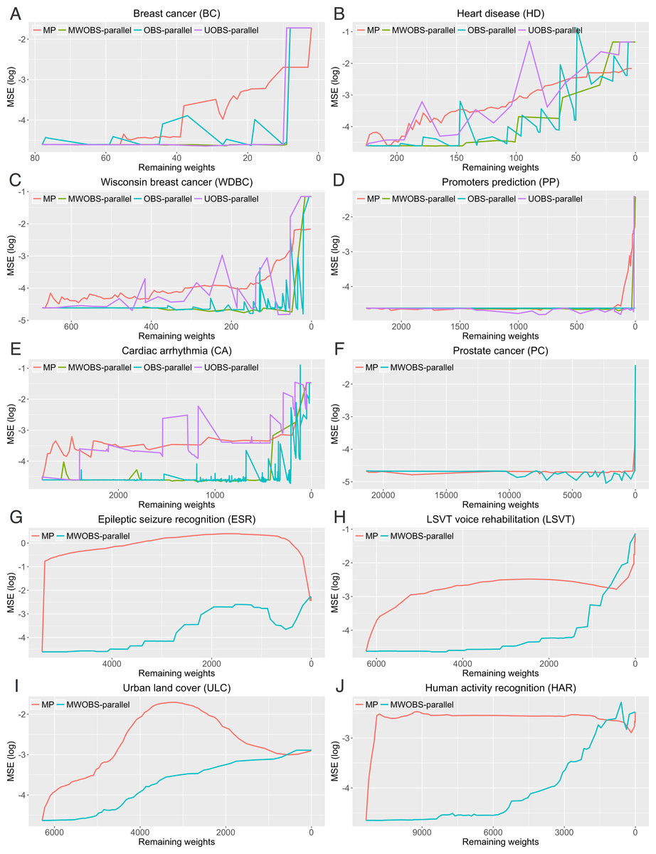
Figure 3: Effects of different pruning algorithms on ANN performance on the training data.
(A–E) Datasets for which all ANN pruning algorithms were completed within a given time limit. (F–J) Datasets for which only MP and MWOBS-parallel algorithms were completed within a given time limit. The x-axis represents the number of remaining weights after each pruning iteration, while the y-axis shows the training MSE.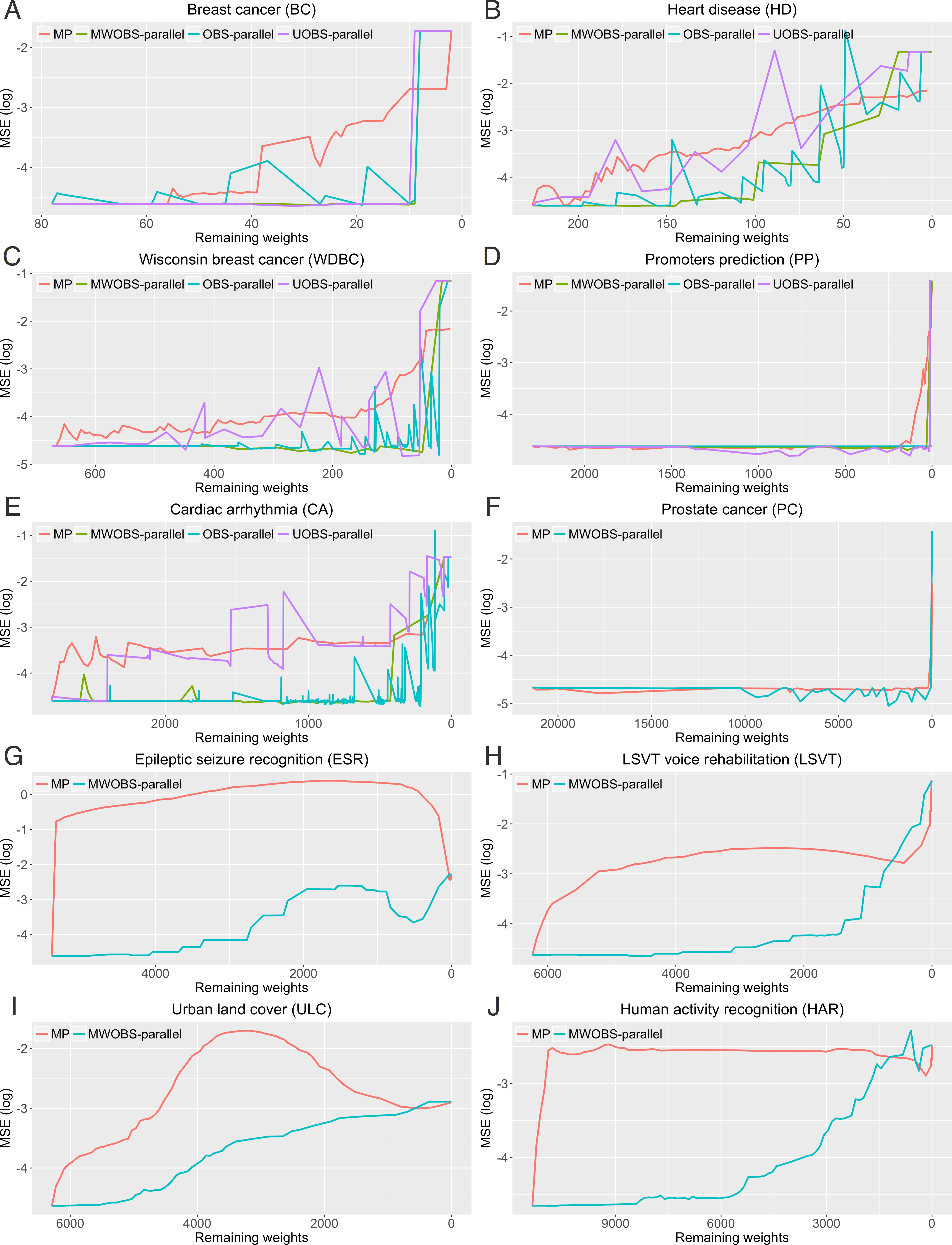
The application of OBS-parallel and UOBS-parallel algorithms is computationally prohibitive for ANNs with a large number of weights (i.e., for datasets with a higher number of input features or ANN with a larger number of nodes in the hidden layer). As such, Figs. 3A–3E show the error curves for all pruning algorithms for smaller datasets (BC, HD, WDBC, PP, and CA) and Figs. 3F–3J and Fig. S1 show the error curves only for MP and MWOBS-parallel algorithms for the remaining 11 datasets (PC, ESR, LSVT, ULC, HAR, SM, TFTF, AID, DCC, SDD, and MD). From these results, we can generally conclude that in order to achieve the greatest reduction of the number of weights, while maintaining the lowest MSE for ANN during the training, the MWOBS-parallel appears to consistently perform better than the other algorithms while being able to cope with more complex ANN structures and datasets.
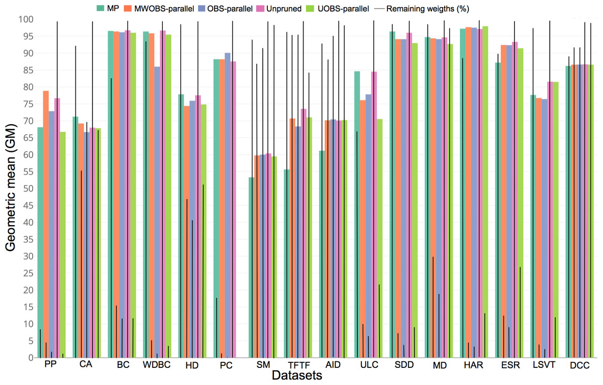
Figure 4: Cross-validation performance and pruning trade-off.
The colored bars represent the GM for each of the datasets, while the solid black line denotes the percentage of the remaining weights in the pruned ANN. The UOBS-parallel results for the PC dataset are not shown as the running time of the algorithm exceeded seven days.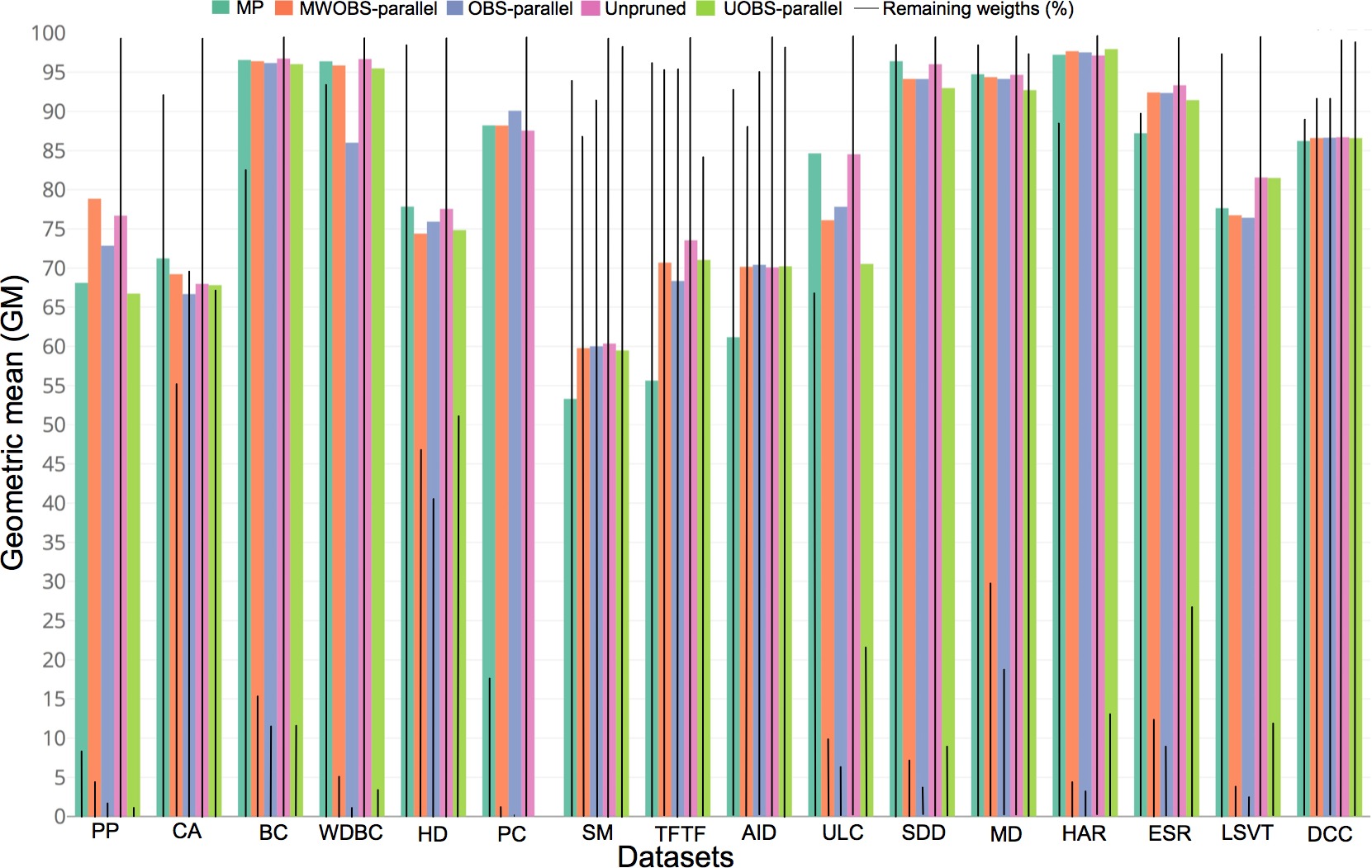
Estimates of model performance and pruning tradeoff
Less complex models are preferred over more complex as this may avoid overfitting the training data, helps increasing model interpretability, and helps reducing computation operations. In ANN specifically, we analyze the effects of ANN pruning on the cross-validation performance (see the Methods section). Figure 4 shows the GM in the cross-validation and the number of weights in the pruned ANNs. Notably, the pruning advantages may be seen in PC dataset, which originally requires a very complex ANN structure as the samples are described by 2,135 input features. For PC dataset, the resulting ANN from the MWOBS-parallel retained ∼400 weights as opposed to 42,740 weights in the unpruned ANN (a reduction of 99% of the weights) with an improvement of 0.65% in the GM. Similarly, for PP and HAR datasets, we observe that MWOBS-parallel reduced the number of weights by ∼95%, while achieving an improved performance with a GM of 78.85%, compared to 76.69% achieved by the unpruned ANN for PP dataset, and 97.68% compared to 97.13% for HAR. The MWOBS-parallel achieved similar results compared to the unpruned ANN but it was able to reduce the number of weights by ∼95%, ∼88%, ∼85%, ∼70%, 13%, 12%, and 8% for WDBC, ESR, BC, MD, SM, AID, and DCC datasets, respectively. Although MWOBS-parallel considerably reduced the number of weights for HD, ULC, and SDD datasets, the MP algorithm achieved better results. Finally, all pruning algorithms achieved worse performance than the unpruned ANN in TFTF dataset with a reduction of ∼2.5% in the GM. Table S2 shows the accuracy, precision, recall, F1 score, Cohen’s kappa coefficient, and the percentage of the remaining weights in the ANN for each dataset. Ideally, we would hope that the pruned ANNs consistently achieve better results than the unpruned ANN. However, the pruning effects are data dependent and may result in ANNs that, depending on the problem, show better, similar or worse performance compared to the unpruned ANNs. In this regard, the Friedman’s test indicates that there is no significant difference (p-value of 0.4663) in the GM performance between the unpruned and pruned ANNs by the different algorithms on our datasets. Nevertheless, the pruned ANNs are considerably simpler, which reduces the computation demands and increases the interpretability of the model. Moreover, the simpler models may arguably perform better for unseen samples, as the simpler models in principle generalize better because they are less likely to overfit the training data.
Overall, results in Fig. 4 show that our solutions are suitable for datasets with a small to a medium number of samples described by a relatively large number of input features. This is frequently the case for many classification problems in real applications. More importantly, MWOBS-parallel can cope with complex ANN structures where other pruning algorithms require considerably longer running times.
ANN pruning effects on data features and comparison to feature selection methods
In addition, we exploit the resulting pruned ANN for assessing and ranking the relevance of the data features. In this regard, we considered the selected features by the ANN pruning and compared their predictive accuracy with seven state-of-the-art methods for FS. Although there have been several attempts to use ANN in FS for certain applications (Becker & Plumbley, 1996; Dong & Zhou, 2008; Kaikhah & Doddameti, 2006; Setiono & Leow, 2000), there are much faster and more efficient approaches for this Guyon & Elisseeff (2003). However, we show that through ANN pruning, we can obtain more insights into the data by ranking and selecting the discriminative features, which is an additional information for users to explore for the problem at hand.
As observed in Fig. 4, pruning algorithms may significantly decrease the number of weights in an ANN. With this reduction, some input features may lose their connecting weights to all nodes in the hidden layer (e.g., x2 in Fig. 1B). This may help to infer the significance of the input features in a dataset. To demonstrate this, we performed pruning for the ANNs derived from the 16 datasets until the MSE exceeded a threshold on the validation data and discarded all input features without weights to the hidden layer. We then re-trained the ANN using only the remaining features to observe how they affected the ANN training and testing performance.
Table 4 shows the GM for the ANNs derived by using the original set of features and the ANNs derived using the subset of features that had at least one connecting weight to the hidden layer after the ANN pruning. Consistent with Fig. 3F, ANN pruning selected only 2% of the features (50 out of 2,135) for PC dataset while improving the GM by ∼1.6% compared to the more complex ANN derived using the original feature set. In general, eight datasets (PC, AID, SM, CA, LSVT, TFTF, HAR, and WDBC) show a considerable reduction of the input features (from 98% to 47%). The achieved GM of the ANN derived using the feature subset from pruning improved in eight datasets (SM, PC, TFTF, AID, ULC, HAR, ESR, and LSVT), remained relatively the same on four datasets (BC, WDBC, DCC, and MD), and decreased in four (HD, PP, CA, and SDD). These results suggest that some classification problems are described with a less redundant set of features, or that the FS methods were not able to discriminate well the redundant from the non-redundant set of features. As such, the negative effects of FS on the GM for HD, PP, CA and SDD datasets indicate that FS may not be useful for all datasets. This may be the case when the data samples are defined by an already small number of highly non-redundant features (as in HD dataset) or simply when the features are weakly or not correlated. Nevertheless, the Wilcoxon signed rank test indicates that ANNs using a reduced feature set perform equally well compared to the unpruned ANNs (p-value of 0.6387), while being considerably simpler and possibly more generalizable.
| Dataset | Remaining input features (%) | GM (%) |
|---|---|---|
| Breast cancer (BC) | 100% (unpruned) | 97.14 |
| 78% (pruned) | 97.14 | |
| Heart disease (HD) | 100% (unpruned) | 80.01 |
| 85% (pruned) | 77.76 | |
| Wisconsin Breast cancer (WDBC) | 100% (unpruned) | 87.38 |
| 53% (pruned) | 87.67 | |
| Promoters prediction (PP) | 100% (unpruned) | 70.71 |
| 70% (pruned) | 57.73 | |
| Cardiac arrhythmia (CA) | 100% (unpruned) | 73.72 |
| 22% (pruned) | 62.64 | |
| Synthetic madelon (SM) | 100% (unpruned) | 59.30 |
| 16% (pruned) | 61.00 | |
| Prostate cancer (PC) | 100% (unpruned) | 92.58 |
| 2% (pruned) | 94.20 | |
| TF-TF combinations (TFTF) | 100% (unpruned) | 73.41 |
| 30% (pruned) | 78.40 | |
| AID886 compounds (AID) | 100% (unpruned) | 66.93 |
| 11% (pruned) | 68.15 | |
| Urban land cover (ULC) | 100% (unpruned) | 78.19 |
| 94% (pruned) | 84.17 | |
| Sensorless drive diagnosis (SDD) | 100% (unpruned) | 96.41 |
| 82% (pruned) | 95.74 | |
| Default credit cards (DCC) | 100% (unpruned) | 88.49 |
| 71% (pruned) | 87.67 | |
| Human activity recognition (HAR) | 100% (unpruned) | 96.61 |
| 42% (pruned) | 97.04 | |
| Epileptic seizure recognition (ESR) | 100% (unpruned) | 91.38 |
| 97% (pruned) | 91.92 | |
| LSVT voice rehabilitation (LSVT) | 100% (unpruned) | 83.20 |
| 24% (pruned) | 87.70 | |
| MNIST digits (MD) | 100% (unpruned) | 94.40 |
| 85% (pruned) | 94.28 |

Figure 5: Performance comparison between the methods for FS and MWOBS-parallel.
(A–P) Cross-validation accuracy results (see the Methods section) obtained from a naïve Bayes classifier derived by using different feature subsets.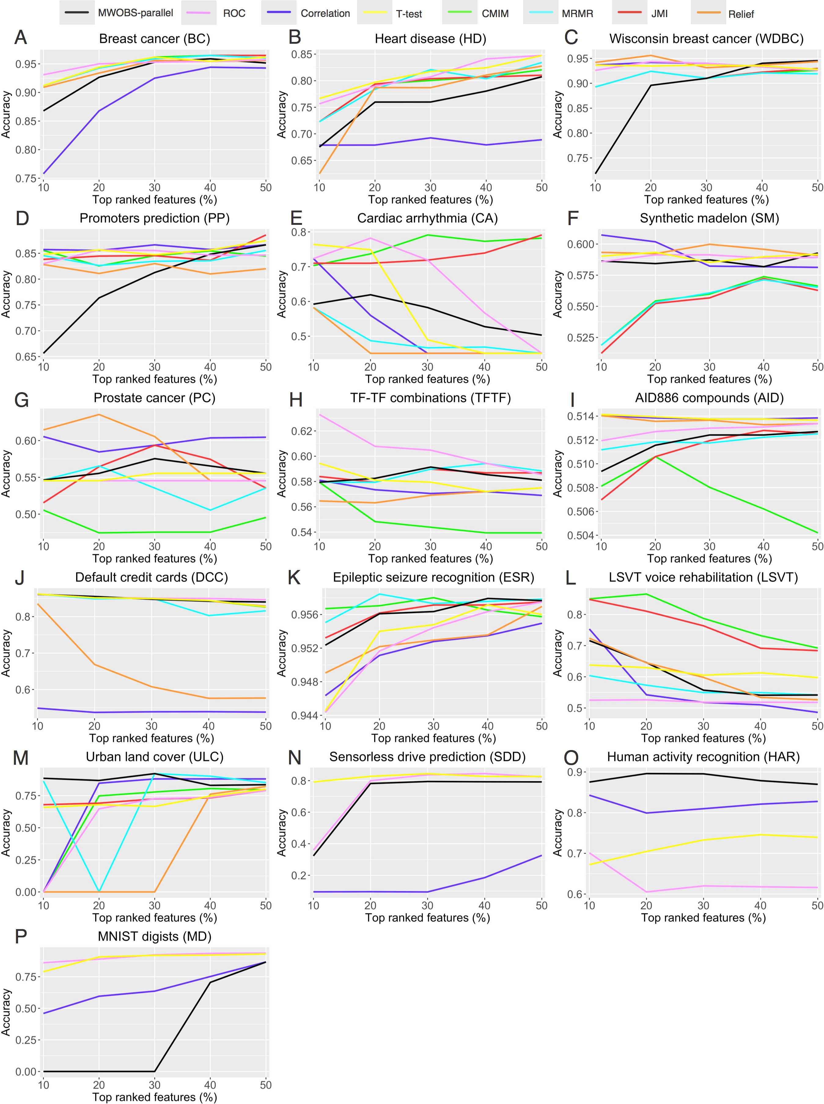
Here, we should note that for nine datasets (WDBC, SM, PC, TFTF, AID, ULC, HAR, ESR, and LSVT) out of 16, the pruned ANNs achieved better performance than the unpruned ANNs. Although the results from Table 4 give an insight of the effects of the FS by ANN pruning, we asked how would this compare to other FS methods. For this, we performed a comprehensive analysis to investigate the ANN pruning effects on the input features using MWOBS-parallel, and compared it with seven state-of-the-art methods for FS.
Figures 5A–5P show the comparison of the cross-validation results obtained from a naïve Bayes classifier derived by using the different subsets of features. Interestingly, when considering 10% or more of the top ranked features, the feature subset determined by MWOBS-parallel outperformed all methods for FS in two datasets (HAR and ULC). Moreover, the feature subset obtained through MWOBS-parallel consistently achieved comparable performance in the remaining datasets compared to the other methods for FS, with WDBC, PP, and MD being the exceptions. Given that many FS methods are heuristics when solving the combinatorial problem of FS, the results obtained by these methods and ANN pruning depends on the dataset and therefore, a specific method may be better than the others for a particular dataset. However, results in Fig. 5 demonstrate that ANN pruning is not only useful for reducing the complexity of the model, but also to get new insights about the data by being able to select and rank the relevant features. We point out that FS through the ANN pruning is a side benefit of the pruning process.
Conclusion
The simplification of ANN structures through pruning is of great importance in reducing the overfitting during the training and in deriving more robust models. Although several ANN pruning algorithms have been proposed, these algorithms are unable to cope with more complex ANN structures in an acceptable amount of time if the performance of the pruned network has to be preserved. The OBS algorithm is among the most accurate pruning algorithms for ANNs. Overall, the main bottleneck of ANN pruning algorithms based on OBS is the computation of the H-inverse for the pruning of each weight. To address this problem, we implemented DANNP, an efficient tool for ANN pruning that implements a parallelized version of the algorithm for faster a calculation of the approximation of the H-inverse. The DANNP tool provides four ANN pruning algorithms, namely, OBS-parallel, UOBS-parallel, MWOBS-parallel, and MP.
We considered 16 datasets from different application domains and showed that mitigation of overfitting using ANN pruning might lead to comparable or even better accuracy compared to fully connected ANNs. Although we have tested our tool on a set of selected datasets, we believe that it is able to cope with problems from different domains and is suitable for small to medium size data regarding the number of features and data instances. We assessed the running times and performance of the implemented pruning algorithms. Our OBS-parallel algorithm was able to speed up the ANN pruning by up to eight times compared to the serial implementation of the OBS algorithm in a 32-core machine. Moreover, we show that MWOBS-parallel produces competitive results to other pruning algorithms while considerably reducing the running time.
Regarding the effects of pruning on the performance, in eight out of the 16 datasets, the pruned ANNs result in a significant reduction in the number of weights by 70% –99% compared to those of the unpruned ANNs. Although results show that the effects of the ANN pruning depend on the dataset, the pruned ANN models maintained comparable or better model accuracy. Finally, we show that through ANN pruning, input features may lose all outgoing weights to the hidden layer, resulting in the selection of features more relevant for the problem in question. We evaluated the selected features from ANN pruning and demonstrated that this set is comparable in its discriminative capabilities as the feature sets obtained by the seven considered state-of-the-art methods for FS. Although FS methods may be used to rank the features based on different statistical measures, we ranked the remaining features considering the sum of the absolute values of their associated network weights. Therefore, the selection of relevant features and the ranking resulting from the ANN pruning provides the user with more information about the classification problem at hand. The DANNP tool can cope with complex and medium size datasets.
Supplemental Information
Pruning algorithms running time in minutes
Cells containing “-” symbol indicate that the algorithm was unable to execute within 48 h.
ANN pruning performance on 16 datasets
This table shows the 10-fold cross-validation results over the 16 datasets; improved F1 score and reduction of the number of weights are indicated in bold. The Unpruned represents the result with non-pruned ANN structure.
Effects of MP and MWOBS-parallel pruning algorithms on the ANN performance
The x-axis represents the number of remaining weights after each pruning iteration, while the y-axis shows the training MSE.