the Creative Commons Attribution 4.0 License.
the Creative Commons Attribution 4.0 License.
 | 11 Dec 2018
Ocean carbon inventory under warmer climate conditions – the case of the Last Interglacial
Augustin Kessler
Eirik Vinje Galaasen
Ulysses Silas Ninnemann
Jerry Tjiputra
During the Last Interglacial period (LIG), the transition from 125 to 115 ka provides a case study for assessing the response of the carbon system to different levels of high-latitude warmth. Elucidating the mechanisms responsible for interglacial changes in the ocean carbon inventory provides constraints on natural carbon sources and sinks and their climate sensitivity, which are essential for assessing potential future changes. However, the mechanisms leading to modifications of the ocean's carbon budget during this period remain poorly documented and not well understood. Using a state-of-the-art Earth system model, we analyze the changes in oceanic carbon dynamics by comparing two quasi-equilibrium states: the early, warm Eemian (125 ka) versus the cooler, late Eemian (115 ka). We find considerably reduced ocean dissolved inorganic carbon (DIC; −314.1 PgC) storage in the warm climate state at 125 ka as compared to 115 ka, mainly attributed to changes in the biological pump and ocean DIC disequilibrium components. The biological pump is mainly driven by changes in interior ocean ventilation timescales, but the processes controlling the changes in ocean DIC disequilibrium remain difficult to assess and seem more regionally affected. While the Atlantic bottom-water disequilibrium is affected by the organization of sea-ice-induced southern-sourced water (SSW) and northern-sourced water (NSW), the upper-layer changes remain unexplained. Due to its large size, the Pacific accounts for the largest DIC loss, approximately 57 % of the global decrease. This is largely associated with better ventilation of the interior Pacific water mass. However, the largest simulated DIC differences per unit volume are found in the SSWs of the Atlantic. Our study shows that the deep-water geometry and ventilation in the South Atlantic are altered between the two climate states where warmer climatic conditions cause SSWs to retreat southward and NSWs to extent further south. This process is mainly responsible for the simulated DIC reduction by restricting the extent of DIC-rich SSW, thereby reducing the storage of biological remineralized carbon at depth.


The Last Interglacial (LIG, or Eemian) is composed of a warm onset around 125 ka characterized by warmer temperature at high latitudes relative to the present and a progressive cooling toward 115 ka when the last glaciation initiated (Masson-Delmotte et al., 2010; Otto-Bliesner et al., 2006). Evidence from land, ice, and ocean records identify the former as the period with the most intense global warming during the last 200 000 years (Capron et al., 2014; Dorthe Dahl-Jensen et al., 2013; Turney and Jones, 2010) mainly due to changes in the orbital configurations. If anthropogenic greenhouse gas emissions continue unabated, a climatically anomalously warm state is expected to occur in the near future with a warming by the end of this century that may be equivalent to the high-latitude reconstructed temperature for the LIG (Otto-Bliesner et al., 2013). The changes in the warm Eemian period may therefore be considered an analog for a future warmer climate.
Few model-based studies examine the carbon cycle dynamics for the LIG period with a particular focus on the ability of models to simulate the transient changes in atmospheric CO2 concentration, which remains relatively stable around 270–280 ppm without displaying any trends (Lourantou et al., 2010; Schneider et al., 2013). Most of these studies provide a better understanding of the land carbon budget, particularly highlighting the importance of temperature changes on the land vegetation and slow processes of CO2 change such as peatland carbon dynamics and CaCO3 shallow-water accumulation (Schurgers et al., 2006; Kleinen et al., 2016; Brovkin et al., 2016). Although there are numerous studies that have analyzed the role of the ocean carbon cycle in regulating the atmospheric CO2, especially for the interglacial-glacial transition period (Menviel et al., 2012; Ridgwell, 2001; Sigman and Boyle, 2000), to the authors' knowledge there is no study that investigate in details changes in marine carbon and nutrient cycling during the Eemian period of the LIG (125–115 ka).
With respect to changes in large-scale ocean circulation, reconstructions indicate that deep Atlantic circulation patterns and water mass geometries likely change over this interval. While mid-depth ventilation of northern-sourced waters (NSWs) is maintained in the North Atlantic by millennial-scale sustained North Atlantic Deep Water formation throughout the LIG (McManus et al., 2002; Mokeddem et al., 2014), southern-sourced waters (SSWs) expanded at depth toward 115 ka (Govin et al., 2009). In addition to large-scale circulation changes, temperature-induced changes in carbon solubility pumps and biological production are expected to alter the ocean carbon budget, in particular in the interior ocean. Other changes such as sea ice extent and ocean ventilation could also affect ocean carbon sequestration rate during the LIG. Elucidating the mechanisms responsible for changes in the ocean carbon distribution and inventory is of interest as it provides past constraints and context for evaluating the response of natural carbon sources and sinks to future climate change. This study aims to fill this knowledge gap by analyzing and comparing, in terms of ocean carbon dynamic, two opposite states of the LIG: the early and warm Eemian onset (125 ka) versus the cooler and late Eemian (115 ka). Using a state-of-the-art Earth system model, our study addresses the regional differences in the ocean carbon storage and the underlying mechanisms.
The paper is organized as follows: in Sect. 2, we describe the model, the experiment design, and the terms and metrics used to quantify the differences in carbon dynamics during the two periods. Section 3 presents the results of the model simulations, while discussions and comparison with previous studies are presented in Sect. 4. Finally, the study is summarized in Sect. 5.
2.1 Model description
The present study uses output of an updated version of the Norwegian Earth System Model (NorESM1-ME), which has recently been further developed to efficiently perform multi-millennial and ensemble simulations (Bentsen et al., 2013; Guo et al., 2018; Luo et al., 2018). This model includes an isopycnal-coordinate ocean general circulation model based on the Miami Isopycnic Coordinate Ocean Model (MICOM; Bleck et al., 1992) and a biogeochemical ocean module adapted from the Hamburg Oceanic Carbon Cycle (HAMOCC5) model (Maier-Reimer, 1993; Maier-Reimer et al., 2005; Tjiputra et al., 2013). The inorganic seawater carbon chemistry in HAMOCC5 includes prognostic partial pressure of CO2 (pCO2) according to the Ocean Carbon-Cycle Model Intercomparison Project (OCMIP) protocols. The pCO2 is computed as a function of temperature, salinity, dissolved inorganic carbon (DIC), total alkalinity (TALK), and pressure. This adapted version of HAMOCC5 does not include prognostic weathering fluxes but does employ a 12-layer sediment model following Heinze et al. (1999), which is particularly relevant for long-term transient simulations. The horizontal resolution of the land and atmospheric components is approximately 2∘, while the ocean and ice components have higher resolutions of approximately 1∘. In the vertical, the ocean model adopts 53 isopycnal layers.
The land component in NorESM (CLM4, Community Land Model version 4) is based on version 4 of the CLM family (Lawrence et al., 2012a). The land surface is sub-gridded into three sub-gridded entities: land units, columns, and plant functional types (PFTs). These sub-gridded cells are used to represent large-scale patterns of the landscape, variability in the soil and snow state variables, and the exchanges between land surface and atmosphere, respectively. Each of the sub-grid entities has its own prognostic variables, is independent, and experiences the same atmospheric forcing. Each cell is averaged and weighted with its fractional area.
The marine ecosystem is based on a nutrient–phytoplankton–zooplankton–detritus (NPZD) model that includes dissolved organic carbon (DOC). The inorganic nutrients consist of three macronutrients (phosphate, nitrate, and silicate) and one micronutrient (dissolved iron). A constant Redfield ratio is adopted in the model as P : C : N : ΔO2 = 1 : 122 : 16 : −172. The phytoplankton growth rate is expressed as a function of temperature, light (Eppley, 1972; Smith, 1936), phosphate, nitrate, and dissolved iron availability, and its loss is regulated by an exudation and mortality rate, in addition to zooplankton grazing. The penetration of light decreases with depth following an exponential function, which responds to a gradual extinction factor formulated as a function of water depth and chlorophyll concentration (Maier-Reimer et al., 2005). The model prescribes a global constant vertical sinking speed of particles produced in the euphotic zone (above 100 m depth). The particulate organic carbon (POC), which comprises dead phytoplankton and zooplankton, sinks through the water column at a speed of 5 m day−1 and is remineralized at a constant rate of 0.02 day−1 when oxygen is available. Other particles such as opal shells and particulate inorganic carbon (PIC) sink at a speed of 60 and 30 m day−1, respectively. Particulates that reach the seafloor without being remineralized interact chemically with the sediment pore water via bioturbation and vertical mixing and advection within the sediment layers. In the model, the air–sea gas exchange of CO2 and O2 only occurs between the ocean surface and the atmosphere in ice-free regions and is computed according to the following three components (Wanninkhof, 1992): the gas solubility in seawater, which is computed as a function of surface salinity and temperature according to Weiss (1970, 1974); the gas transfer velocity, which is proportional to the square of the surface wind speed and is computed as a function of the Schmidt number; and finally the air–sea gradient of gas partial pressures. To better elucidate various biogeochemical processes on the carbon cycle, the model is updated to also include preformed O2, TALK, and PO4 tracers in the biogeochemical module. At the surface, these preformed tracers are set to their non-preformed value and are advected passively by the ocean circulation in the interior without any other sources and sinks. Finally, in order to provide information of the water mass ages since its last contact with the atmosphere, an idealized age tracer is implemented and simulated in the NorESM model. Hence, the age tracer is set to zero for all water masses at the ocean surface and subsequently transported and mixed passively with circulation in the ocean interior and integrated with the model time step. This tracer is also used to estimate the ventilation rate of different interior water masses.
2.2 Experiment setup
Two equilibrium experiments are performed over the Eemian (model data available at https://doi.org/10.11582/2018.00038; Kessler, 2018), one near the onset (warmer than today, 125 ka) and one at the end (colder, 115 ka) of the Last Interglacial. Both experimental configurations follow the standard protocols of the third phase of the Paleoclimate Modelling Intercomparison Project (PMIP3; https://pmip3.lsce.ipsl.fr/, last access: 5 December 2018), with a fixed vegetation coverage from the preindustrial boundary conditions. The only differences from the preindustrial configurations are the orbital parameters and the greenhouse gases concentrations (CO2, CH4, N2O). For the experiment at 125 ka (115 ka), the atmospheric CO2, CH4, and N2O levels are prescribed to be 276 ppmv (273 ppmv), 640 ppb (472 ppb), and 263 ppb (251 ppb), respectively. The two experiments are branched off from 1000 years of spin-up with a preindustrial setup and forced with their respective interglacial boundary conditions for 4000 simulation years.
In the last 50 years of Eemian forcing simulations the ocean is close to equilibrium. Only small drifts remain, mainly in the Pacific basin where the equilibrium is still not fully established. Therefore, the global ocean DIC and TALK slightly decrease in the experiment at 125 ka (115 ka) by approximately −0.15 PgC yr−1 (−0.06 PgC yr−1) and −0.01 Pmol yr−1 (−0.01 Pmol yr−1), respectively. However, these drifts are small compared to the absolute ocean budget in DIC (37391 and 37 705 PgC) and TALK (3291 and 3303 Pmol) for the 125 and 115 ka experiments, respectively. The differences in the pCO2 and TALK budget are small between the two experiments. Such changes would affect the DIC budget by about 32 PgC. The CO2 flux is relatively constant and depicts the ocean as a weak source to the atmosphere with an outgassing of 0.12±0.06 at 115 ka and 0.15±0.06 PgC yr−1 at 125 ka. In addition, the difference in sedimentation rates between the two experiments ( PgC) appears to be negligible compared to the difference in DIC budget.
2.3 DIC decomposition
In order to analyze the oceanic carbon cycle, dissolved inorganic carbon (DIC) is decomposed into its preformed and biological components (Eq. 1), following Bernadello et al. (2014):
The preformed component of DIC (DICpre) comprises saturated and disequilibrium parts (Eq. 2).
where the DIC at saturation (DICsat) describes the DIC concentration when the water parcel is in full equilibrium with the atmospheric CO2 when it is last in contact with the surface. In our model, changes in DICsat are mainly affected by changes in preformed TALK. We compute this variable offline with the inorganic carbon chemistry program CO2SYS developed in Matlab (van Heuven et al., 2011), including other parameters such as the model output of preformed alkalinity (TALKpre), preformed phosphate (PO4pre), surface silicate, salinity, and temperature. In addition, the atmospheric CO2 concentration from each experiment is used. To complete the CO2SYS input, we applied the dissociation constants K1 and K2 introduced by Mehrbach et al. (1973) and refitted by Dickson and Millero (1987). The disequilibrium part of DIC (DICdis) measures the disequilibrium state of the surface water with respect to the atmosphere. This parameter is computed from the DICtot (output), from which the biological and saturated DIC components (DICbio and DICsat) are subtracted. Therefore, all components are included in its calculation. A negative DICdis occurs when the water parcel sinks into the ocean interior before a full equilibration with the atmosphere is obtained, which leads to an undersaturation of the water parcel. This undersaturation can also be reinforced by biological CO2 consumption at the surface, which tends to increase the timescale needed for the water parcel to equilibrate. However, a positive DICdis translates into a supersaturation. The latter occurs when deep waters, which contain high concentration of DIC because of remineralization processes, upwell or mix vertically with the surface waters (Follows and Williams, 2004). Both DICdis and DICsat are transported by ocean circulation into the interior ocean.
The biological component of DIC comprises (1) the interior remineralization of organic matter (expressed in carbon), which is produced in the euphotic layer via photosynthesis (also referred to as soft-tissue pump), and (2) the remineralization of planktonic calcium carbonate shells (expressed in carbon; calcium carbonate pump). These two remineralization components are added to form the biological component of DIC, as shown in Eq. (3).
The remineralization of soft tissues (hereafter DICsoft) contributes via phosphate (PO4) remineralization through a carbon phosphorus stoichiometric ratio . This component is calculated from the difference between the total and the preformed PO4 according to
The carbonate pump contributes through the dissolution of CaCO3 hard shells, calculated as difference between the total and the preformed alkalinity and PO4 following
where is the Redfield ratio adopted by the model and the phosphate term accounts for the alkalinity changes owing to the soft-tissue pump.
In our analysis, we show differences between the warmer 125 ka and the colder 115 ka experiments. We therefore use the delta notations ΔDICtot, ΔDICsat, ΔDICsoft, ΔDICcarb, and ΔDICdis to refer to changes between the warmer and the colder periods.
2.4 Water mass analysis
In order to identify water mass sources, we apply the “PO” tracer as defined by Broecker (1974). It is computed using phosphate and oxygen fields following
where is the phosphorus-to-oxygen stoichiometric ratio used in the model. This tracer is presumed to be nearly constant for a specific water mass. It is based on the principle that phosphate is released while oxygen is used during remineralization, and vice versa during biological production. The distinction of water masses using PO is useful for contrasting water masses with very different surface PO values. Here, we mainly use PO to identify NSW and SSW masses in the deep ocean below 1000 m depth characterized by low and high PO values, respectively.

Figure 1Difference in sea surface temperature (ΔSST) between 125 and 115 ka. Only significant differences (i.e., with absolute value greater than the interannual standard deviation over the last 50 years in both 125 and 115 ka) are shown. The green and purple lines correspond to 50 % sea ice extent at 115 and 125 ka, respectively. The black (blue) thick lines depict regions affected by a deepening (shallowing) of the mixed-layer depth (with difference greater than 100 m depth) at 125 ka compared to 115 ka.
Section 3.1 describes the sea surface temperature and sea ice changes, while changes in water mass properties are discussed in Sect. 3.2. The near-surface changes that particularly influence the biological pump are addressed in Sect. 3.3, and global to regional oceanic DIC storage changes are presented in Sect. 3.4. The analysis is performed over the average of the last 50 years of the simulations. In addition, the global ocean is divided into three main basins: Atlantic, Indian, and Pacific.
3.1 Sea surface temperature and sea ice
Our model simulates a global and annual increase of sea surface temperature (SST; +0.27 ∘C) at 125 ka relative to the 115 ka experiment. This warming is mainly simulated at high latitudes (Fig. 1a–d) where higher SSTs are simulated throughout the year in the Southern Ocean (SO), south of Greenland, the Norwegian Sea, and the northern part of the Pacific Ocean. This persistent warming at 125 ka induces the sea ice to melt (Fig. 1, green and purple lines). Consequently, in the areas where sea ice extent is reduced, there is more air–sea gas exchange and an increase in mixed-layer depth (MLD; Fig. 1, black lines in the Southern Ocean). In the Labrador Sea the mixed layer depth at 125 ka is deeper by more than 100 m than at 115 ka. This is due to higher salinity simulated in this region at 125 ka. At lower latitudes, the SSTs vary more spatially and seasonally. For example, in some parts of the Atlantic Ocean (North Atlantic Drift, the equatorial region, and some sections of the subantarctic near the 45∘ S band) cooler SSTs are simulated over several seasons (ΔSST<0, Fig. 1a–b). While the North Atlantic drift depicts cooler SSTs during boreal winter and spring (Fig. 1a–b), colder SSTs last until the boreal summer in the equatorial region of the Atlantic Ocean (Fig. 1a–c). The 45∘ S latitude band remains cooler over the four seasons. Here, the MLD seems to be more controlled by changes in salinity instead of temperature distribution.
We note that relative to the preindustrial, based on proxy (Hoffman et al., 2017), our model simulates consistent spatial feature of annual SST anomalies at 125 ka. It simulates, among other things, (i) strongest warming at high latitudes, specifically in parts of the Southern Ocean; (ii) weak cooling at low latitudes; (iii) cooler SST in most of the Indian Ocean; and (iv) a warmer eastern North Pacific. Nevertheless, the amplitude of SST warming and cooling at specific sites tends to be weaker in our model. This feature appears to be common in other global models and could be attributed to their low spatial resolutions (Hoffman et al., 2017).
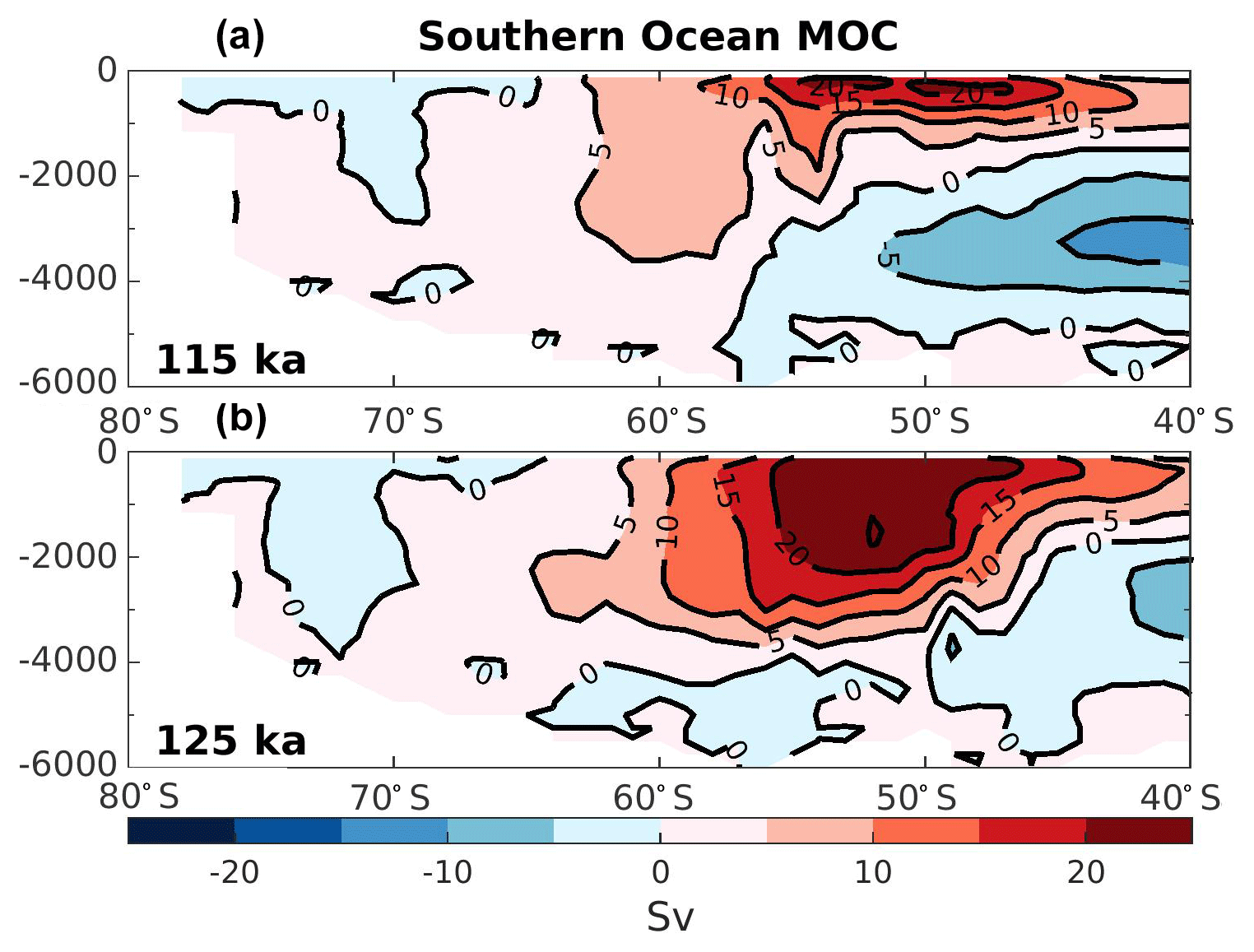
Figure 2Southern Ocean overturning stream function in Sverdrup (Sv) for the experiment at 115 ka (a) and 125 ka (b). Red colors represent water masses moving clockwise, while blue colors represent water masses moving counterclockwise.
3.2 Water mass properties
In order to analyze the water mass properties, it is useful to examine the changes in the overturning circulation. Figure 2 shows the global overturning stream function in the Southern Ocean for both experiments. The Antarctic circumpolar current is simulated stronger and deeper at 125 ka compared to 115 ka (Fig. 2). This strengthening mainly occurs in the Pacific section of the Southern Ocean (near 50∘ S), suggesting an increase of the ventilation rate of the intermediate waters formed in this region. The Atlantic section of the Southern Ocean remains weakly modified. Indeed, using the same model simulations as the present study, Luo et al. (2018, Supplement Fig. S8) show that the surface wind speed in the eastern and western South Atlantic are relatively similar at 125 and 115 ka. In addition, they also show that the simulated Atlantic Meridional Overturning Circulation (AMOC) at 125 ka is as vigorous as at 115 ka but deepen by about 300 m depth. This suggests that the mid-depth and bottom water in the North Atlantic Ocean should be better ventilated at 125 ka than at 115 ka.
These changes in the overturning circulation affect the water mass age tracer. Analyzing this parameter allows us to examine the interior ocean ventilation rate. A reduction in water mass age translates to a faster ventilation rate and vice versa for an increase in age. The differences in water mass age between 125 and 115 ka are presented in Fig. 3, depicting the zonally averaged sections for each ocean basin. The water mass ages in the Atlantic and the Indian oceans show similar patterns, with mean older water masses in the upper layers at 125 ka (roughly +100 years) and younger water masses below 1000 m depth (as much as 500 years younger). This is consistent with a deeper and slightly stronger AMOC at 125 ka as shown in Luo et al. (2018). The Southern Ocean (south of 50∘ S) contains younger water masses throughout the entire water column in both basins at 125 ka, translating to a stronger ventilation rate. This is likely due to changes in the distribution of SSW and NSW. Figure 4 show that there is a clear distinction between interior water mass structure in the Atlantic basin between 115 ka (Fig. 4a) and 125 ka (Fig. 4c). It shows that below 2000 m depth the SSW retreats further southward at 125 ka relative to 115 ka in the Atlantic basin. This confinement in SSW is induced by the change in the Antarctic sea ice cover (Fig. 1), as explained by Ferrari et al. (2014). However, the model also simulates a modification in SSW density (−0.2 kg m−3 at 125 ka compared to 115 ka; Fig. 4a, c). This reduction in water density is mainly driven by the input of low-salinity freshwater from the melting of the Antarctic sea ice and may have an additional impact on determining the Atlantic distributions of NSW and SSW. As a result of sea ice retreat, the winter mixed layer depth in this area increases, resulting in younger water mass age in the Southern Ocean. Near the surface (∼ 800 m depth) the SSW seems to enter further north in the Atlantic basin at 125 ka (Fig. 4c) relative to 115 ka (Fig. 4a).
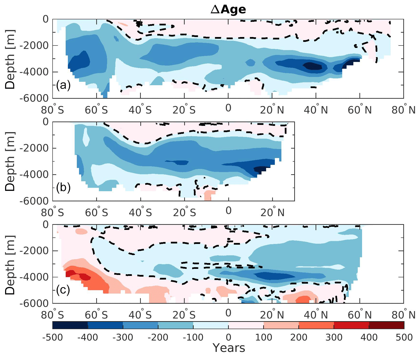
Figure 3Zonally averaged section of the difference in water mass age (ΔAge) between 125 and 115 ka in (a) the Atlantic Ocean, (b) the Indian Ocean, and (c) the Pacific Ocean. The dashed lines display ΔAge=0.
While such large redistributions of northern- and southern-origin deep waters only occur in the Atlantic, these changes also influence water properties in the Indian Ocean due to the “downstream” advection of younger deep water into the interior during the warmest period (125 ka – Fig. 3b). In addition to simple advection of younger water northward in the Indian basin, the residence time of the Indian Ocean's deep water must also decrease since the ventilation ages decrease northward at depth. By contrast, in the Pacific Ocean, the zonally averaged bottom-water mass ages are simulated to be older at 125 ka (Fig. 3c). However, this basin can be divided between the western and eastern side. While the western side is also influenced by the younger water masses created in the Atlantic Ocean, the eastern side waters of the basin are simulated to be older at 125 ka by as much as 300 years. These older water masses are created in the Pacific SO and may be affected by a flattening of the isopycnals south of 60∘ S at 125 ka (Fig. 4d, gray lines). This flattening of the isopycnals is influenced by both sea ice melting and higher SSTs, and suggests stronger stratification and a weaker subduction rate. In addition, the SSW boundary (Fig. 4b, d; light purple dashed lines) seems to be slightly poleward at 125 ka ( S) compared to 115 ka ( S). This may suggest that more surface water originating from the subtropical gyre (more depleted in phosphate) enters the Pacific section of the Southern Ocean. Finally, the Pacific intermediate waters are simulated as younger at 125 ka when compared to 115 ka (Fig. 3c), which is consistent with the strengthening of the upper cell of the overturning circulation previously mentioned for this region.
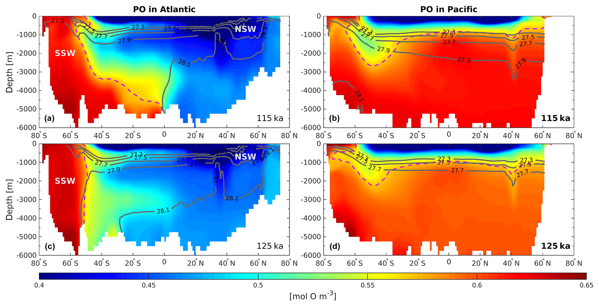
Figure 4Zonally averaged section of PO as defined by Broecker (1974) in (a, c) the Atlantic Ocean at 115 and 125 ka, respectively, and (b, d) the Pacific Ocean at 115 and 125 ka, respectively. The light purple dashed lines delimit the water influenced by the SSW from water influenced by the NSW. The dark gray solid lines depict the neutral density (units: kg m−3).
Table 1Difference in southern-sourced water (ΔSSW) in the global ocean and for each basin. Row 1 shows the volume (VSSW) according to our PO ≥0.57 mol O m−3 criteria. Rows 2 and 3 summarizes the DIC and water mass age mean value for the two period of study. The changes relative to 115 ka are given as a percentage in parenthesis.
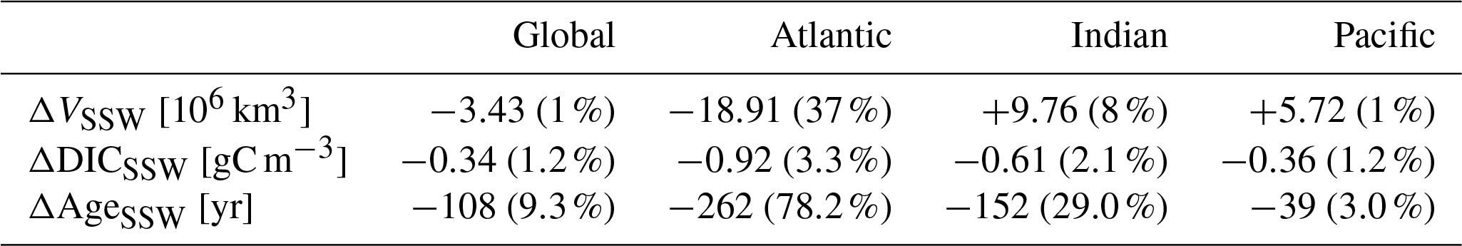
The southern-sourced waters are particularly affected in terms of geometry distribution. We therefore divide the changes from these SSWs into the three basins. Table 1 summarizes the changes occurring below 1000 m depth in the SSWs in terms of volume, DIC, and water mass age for each basin and reveals the Atlantic as the most affected area under warmer climate conditions. The relative difference in all those three characteristics (ΔVSSW, ΔAgeSSW, and ΔDICSSW) between 125 and 115 ka is the greatest in the Atlantic (−37 %, −262 years, and −0.92 g C m−3). This demonstrates that the ventilation mechanism in the Atlantic sector of the SO is likely to be more sensitive (than in other basins) to climate change.
In response to the different forcings between 125 and 115 ka, significant changes are simulated in deep-water ventilation rates and water mass distribution in the three basins. While the responses in the Atlantic and Indian oceans have some similarity (better deep-water ventilation), the Atlantic basin seems to be the most sensitive and also simulates water mass geometry changes. However, the ventilation rate in the Pacific Ocean depicts an opposite sign of change to that of the Atlantic and Indian oceans. In the next section we discuss how these modification impact the near-surface productivity in our model.
3.3 Near-surface productivity
Figure 5 shows the differences in carbon export production (EPC) and phosphate (PO4) at the surface of the ocean between 125 and 115 ka. When comparing the 125 and 115 ka experiments, our model simulates two major features characterized by (i) an increase in EPC in the equatorial region of the Atlantic Ocean (Fig. 5a, turquoise rectangle) and (ii) a reduction in EPC of similar magnitude in the equatorial region of the Pacific Ocean (Fig. 5a, purple rectangle). Although there are changes in surface wind speeds and vertical mass fluxes (not shown here) in the equatorial regions, they do not consistently explain the simulated changes in export production (i.e., stronger wind and upwelling in the eastern equatorial Pacific at 125 ka compared to 115 ka, where a decrease in export production is simulated; in parts of the equatorial Atlantic some increase in export production may be related to the simulated stronger upwelling at 125 ka). However, nutrient changes in the Atlantic and Pacific sections of the Southern Ocean are consistent with the changes in export production, and therefore we suggest the following mechanism. In the Atlantic Ocean, the subantarctic water (45∘ S latitude band) corresponds to the southern-sourced intermediate water formation in the model. This water mass sinks and reemerges along the Equator (Fig. 5, turquoise rectangles). This pattern expected from models and modern observations shows that the intermediate and mode waters formed at high southern latitudes feed the subtropical thermocline and act as a predominant source of nutrients important for sustaining low-latitude biological productivity (Gu and Philander, 1997; Sarmiento et al., 2004b). We acknowledge that there is uncertainty in the complex pathways of the subantarctic water masses toward the Equator simulated in the model. Nevertheless, due to higher preformed and remineralized phosphate in the subantarctic water sinking region, more PO4 is advected through this “ocean tunnel” to the Equator and therefore leads to an increase in EPC (Fig. 5a, turquoise rectangle). A similar ocean tunnel (Fig. 5, purple rectangle) connects the high and low latitudes in the Pacific Ocean but results in the opposite sign of change. Here, as pointed out in Sect. 3.2, more subtropical waters seem to enter the Pacific Southern Ocean at 125 ka than at 115 ka. These waters are depleted in phosphate compared to southern-sourced waters. As a result, less phosphate is subducted toward the equatorial Pacific (Fig. 5b, purple rectangle), leading to a reduction in the EPC near the equatorial upwelling (Fig. 5a, purple rectangle).
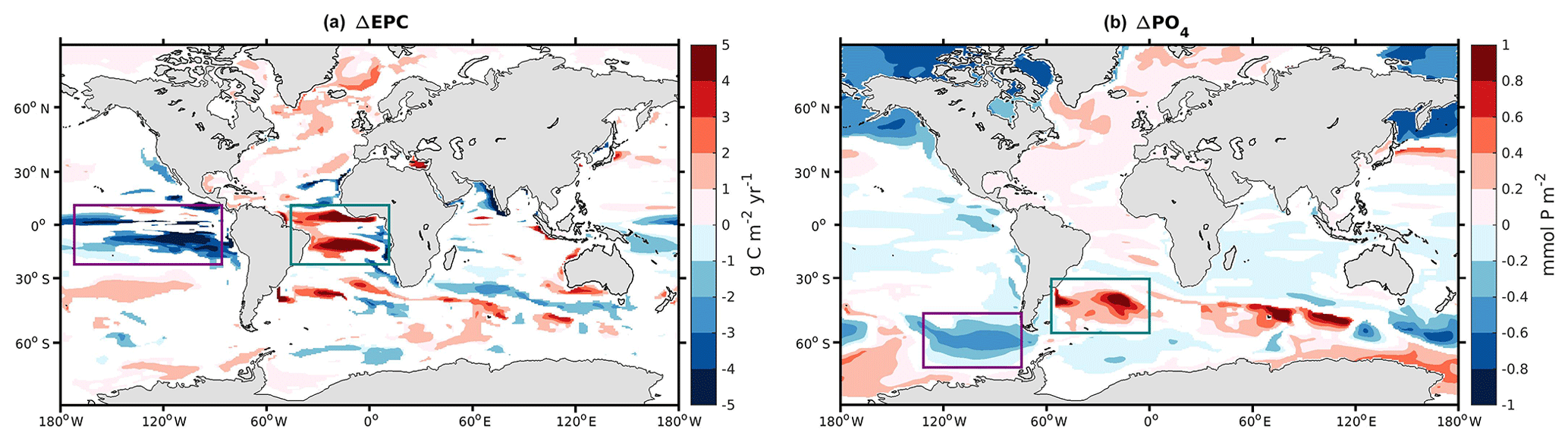
Figure 5Difference in (a) export production of carbon at 100 m depth (ΔEPC) and (b) phosphate at the surface (ΔPO4) between 125 and 115 ka. When the absolute value of the difference is below the standard deviation over the last 50 years at 125 and 115 ka, the value returns a NaN. Purple and turquoise rectangles highlight the two “ocean tunnels” linking the sinking/upwelling regions of southern-sourced intermediate waters in our model.
There are no significant changes in the biological activity in the Indian Ocean or the remaining Southern Ocean. Only a weaker carbon export at 125 ka relative to 115 ka is simulated around 40∘ S and the Arabian Sea.
Thus, the simulations reveal that changes in Southern Hemisphere thermocline ventilation regions modulate basin scale productivity and export production even within an interglacial period with modest changes in external forcing. This result is broadly consistent with previous studies suggesting that the upper limb of the biogeochemical divide is critical for setting biological export production and is sensitive to climate changes (Marinov et al., 2006; Moore et al., 2018; Sarmiento et al., 2004a). Despite zonally homogeneous forcing we find a basinally heterogeneous response both in subantarctic ventilation and in low-latitude productivity which is similar to, albeit more extreme than, the basin specific response simulated for future warming and stratification (Moore et al., 2018).
These changes in surface physical and biological activities could also have implications for the exchanges of carbon between near-surface and interior water masses, and therefore the interior carbon budget. In the next section, ventilation changes at 125 ka are compared to 115 ka by analyzing the simulated water mass properties.
3.4 Global and regional carbon budgets
Figure 6 shows the difference in the carbon inventory vertical profiles between 125 and 115 ka as simulated by our model. The changes in DICtot, DICsat, DICsoft, DICcarb, and DICdis are averaged over a 500 m depth interval. The global amount of DICtot is −314.1 PgC in the ocean under the warmer conditions (Fig. 6a, gray ΔDICtot). Since the atmospheric CO2 is kept constant in each experiment, this carbon loss at 125 ka compared to 115 ka is implicitly assumed to be balanced out by the changes in the land carbon reservoir. Here, the Atlantic Ocean accounts for 15 % (−49.1 PgC) of that global decrease, while the Indian and the Pacific basins contribute 28 % (−87.2 PgC) and 57 % (−179.0 PgC), respectively. Only in the near-surface layers does the model simulate a positive ΔDICtot, which translates to higher surface DIC concentration at 125 ka relative to 115 ka. Most of the ocean interior has lower DIC concentration at 125 ka, with the strongest difference in ΔDICtot simulated between 2000 and 3000 m depths for each basin, except for the Atlantic (Fig. 6b–d). The soft-tissue pump and the disequilibrium effect are the main contributors for the reduced carbon inventory depicted at 125 ka at the global scale (Fig. 6a, green and purple bars) – each accounting for a third of the total −314.1 PgC decrease. Similarly, ΔDICtot in the Atlantic basin is also predominantly controlled by the biological pump, i.e., the soft-tissue plus carbonate pump throughout the entire water column with a decrease at depth and an increase in the near-surface (Fig. 6b). Except for the upper ocean, the contribution from the saturation component related to temperature and salinity change is generally negligible.
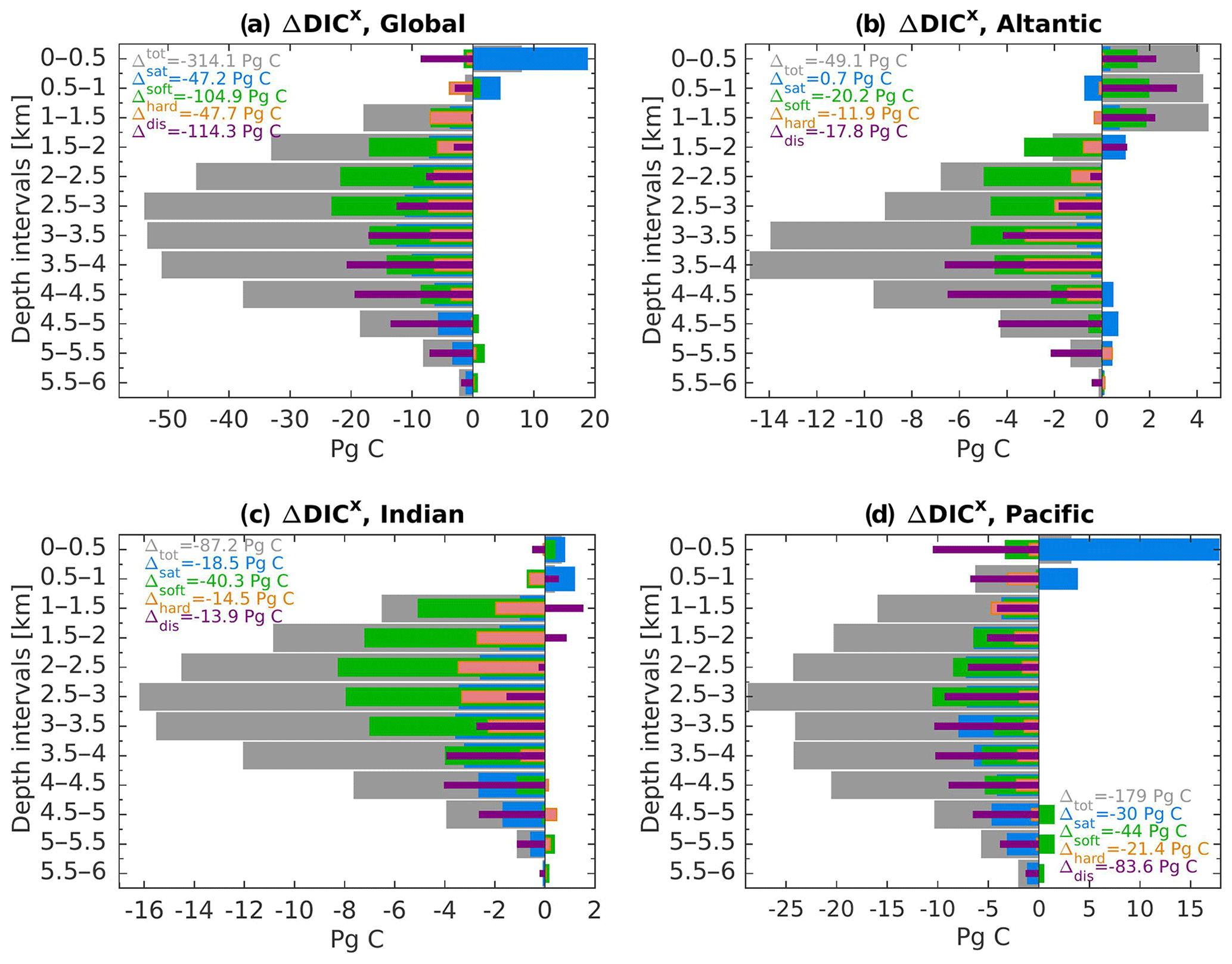
Figure 6DIC differences between 125 and 115 ka (ΔDICx) in (a) the global ocean and the (b) Atlantic, (c) Indian, and (d) Pacific basins. The ΔDICx is averaged over a 500 m depth interval where “x” refers to the different components of the DIC. The DICtot is represented by the gray bars and is decomposed into its four components: ΔDICsat (blue), ΔDICsoft (green), ΔDICcarb (orange), and ΔDICdis (purple). The sum throughout the water column of each components is given by the legend.
The ΔDICtot of the Indian basin also depicts a strong reduction at 125 ka relative to 115 ka. Here the soft-tissue and saturation components simulate the strongest decrease (Fig. 6c, green and blue bars). In addition, near-surface changes in ΔDICtot are controlled by the changes in ΔDICsat. Similarly, the near-surface layer of the Pacific Ocean is also controlled by the changes in the saturation component (Fig. 6d), simulating a positive difference of about +18 PgC. Changes in the deeper layers are mainly attributed to the disequilibrium effect and the soft-tissue pump, accounting for a decrease of −83.6 and −44.0 PgC at 125 ka relative to 115 ka, respectively. However, the saturation component also has a considerable influence on the carbon storage with persistent negative ΔDICsat throughout the water column.
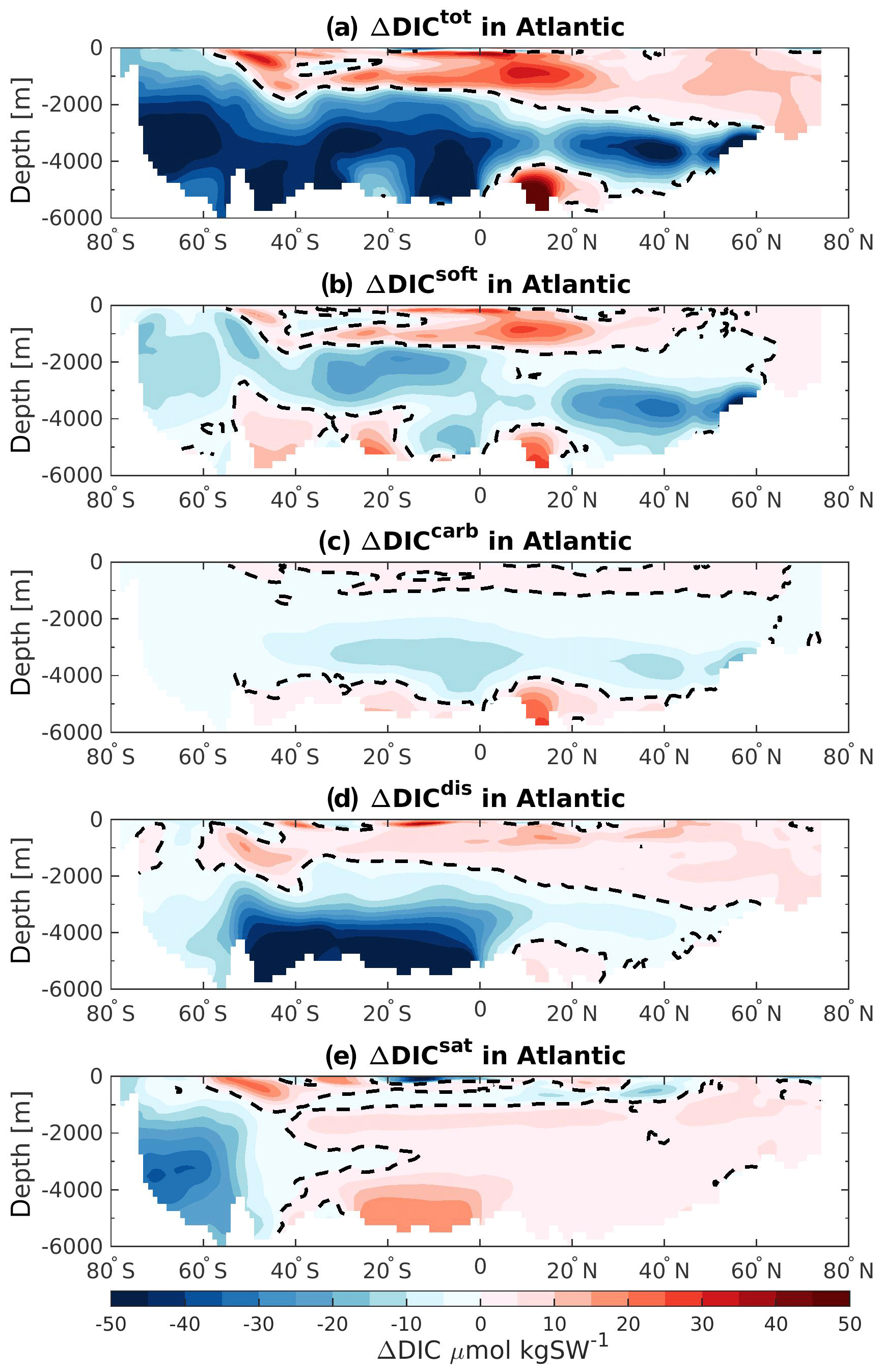
Figure 7Atlantic zonally averaged section of the difference in (a) ΔDICtot, (b) ΔDICsoft, (c) ΔDICcarb, (d) ΔDICdis, and (e) ΔDICsat between 125 and 115 ka. The black dashed lines represent the zero values.
In order to address the regional changes, we analyze the differences in each DIC components further by calculating the zonally averaged values in each basin. Figures 7, 8, and 9 depict these differences for the Atlantic, Indian, and Pacific basins, respectively. As shown in Fig. 6b, the carbon inventory of the Atlantic is reduced mainly below 1500 m depth. Here the Southern Hemisphere is the most affected region, which depicts the strongest differences in ΔDICtot (Fig. 7a, blue shading). This pattern corresponds well to the changes in soft-tissue pump (Fig. 7b). Near the surface, higher carbon export (Fig. 5a) increases the remineralization of organic matter, leading to higher DIC concentration at 125 ka. At depth, the slightly deeper AMOC at 125 ka (compared to 115 ka), leads to better-ventilated mid-depth to bottom waters in the Northern Hemisphere, leading to less remineralized organic matter by reducing the water mass age. This is reflected by the negative ΔDICsoft and ΔDICcarb, translating to a less effective soft-tissue and carbonate pump at 125 ka. Positive changes in ΔDICtot in near-surface waters and bottom water at 20∘ N also arise from the soft-tissue and carbonate signal due to the increase of the alkalinity (not shown here) and slightly older water masses along the African coast. The bottom waters in the Southern Hemisphere are mainly controlled by a stronger disequilibrium effect, i.e., negative change in comparison to 115 ka. This change in disequilibrium is due to the sea-ice-induced retreat of the SSW and the inflow of more NSW between 50∘ S and the Equator at 125 ka. The NSW mass, formed in the North Atlantic, is generally more subject to biological production during its near-surface northward transport before sinking into the interior than the SSW (Duteil et al., 2012). The biological production consumes DIC during photosynthesis and pushes the water mass further out of the equilibrium with the atmospheric CO2, inducing ΔDICdis to be more negative. The negative values of ΔDICdis are conserved when the water parcel flows southward into the deep ocean. For this reason, the regions that are no longer influenced by SSW at 125 ka depict a negative ΔDICdis (Fig. 7d). However, the upper layers of the Atlantic Ocean are mostly simulated with higher DICdis (positive ΔDICdis, or less disequilibrium at 125 ka). This could be induced by more SSW (less disequilibrated than NSW) entering the Atlantic basin further north near the surface as Fig. 4c suggests. Finally, the loss of carbon in the Southern Ocean is shown to be mainly attributable to a decrease of the saturation component at 125 ka. This decrease is mainly attributed to lower TALKpre (not shown here), possibly provoked by the melting of the sea ice.
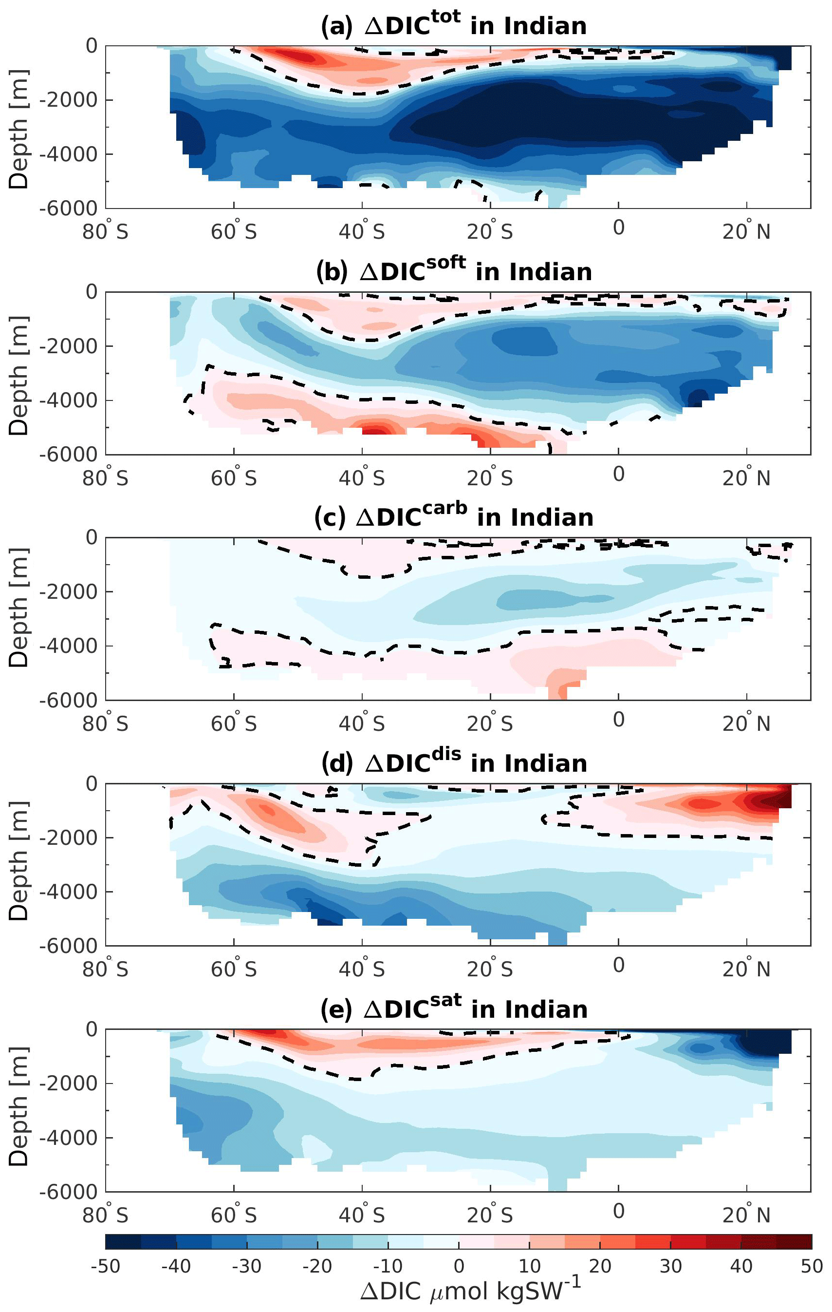
The DIC storage in the Indian Ocean generally shows a decrease at 125 ka, with the strongest changes occurring at depth north of 30∘ S (Fig. 8a, dark blue shading). Positive ΔDICtot are nevertheless simulated in the region that may correspond to the Antarctic Intermediate Water (AAIW) (Fig. 8a, red shading). Similar to the Atlantic basin, the pattern of the soft-tissue pump changes corresponds to the ΔDICtot pattern throughout most of the Indian Ocean. This decrease in biological remineralization is in agreement with the water mass age changes seen in Sect. 3.2 (Fig. 3b): younger water masses account for less biologically induced DIC content. However, the bottom and the surface waters show opposite signs in the ΔDICtot, which suggests that other processes are acting in these regions. The differences in the carbonate pump remain small and roughly follow the pattern of the soft-tissue pump (Fig. 8c). Changes in the bottom-water ΔDICtot can be attributed primarily to the difference in the disequilibrium effect, which is probably affected by larger influence of NSW at 125 ka relative to 115 ka as described for the Atlantic basin, and to a slight reduction in the saturation component. In addition, the disequilibrium component might also be influenced by stronger carbon export in the Southern Ocean (as the positive ΔDICsoft and Fig. 5a suggest). The strong positive ΔDICdis simulated near the surface along the Indian coast is in good agreement with lower SSTs (Fig. 1a–c) allowing more DIC to be absorbed at 125 ka and a strong reduction in carbon export production (Fig. 5a). Finally the negative ΔDICsat depicted in the top layers in the north of the Indian Ocean is mainly attributed to a change in water mass origin from 115 to 125 ka. During 115 ka the SSW upwells from the deep ocean into the Arabian Sea. By contrast, at 125 ka, the waters coming from the Indonesian region mix with SSW. These Indonesian throughflow water masses initially coming from the Pacific Ocean are affected by strong precipitation in the Indonesian basin, which reduces the TALK at the surface and therefore DICsat.
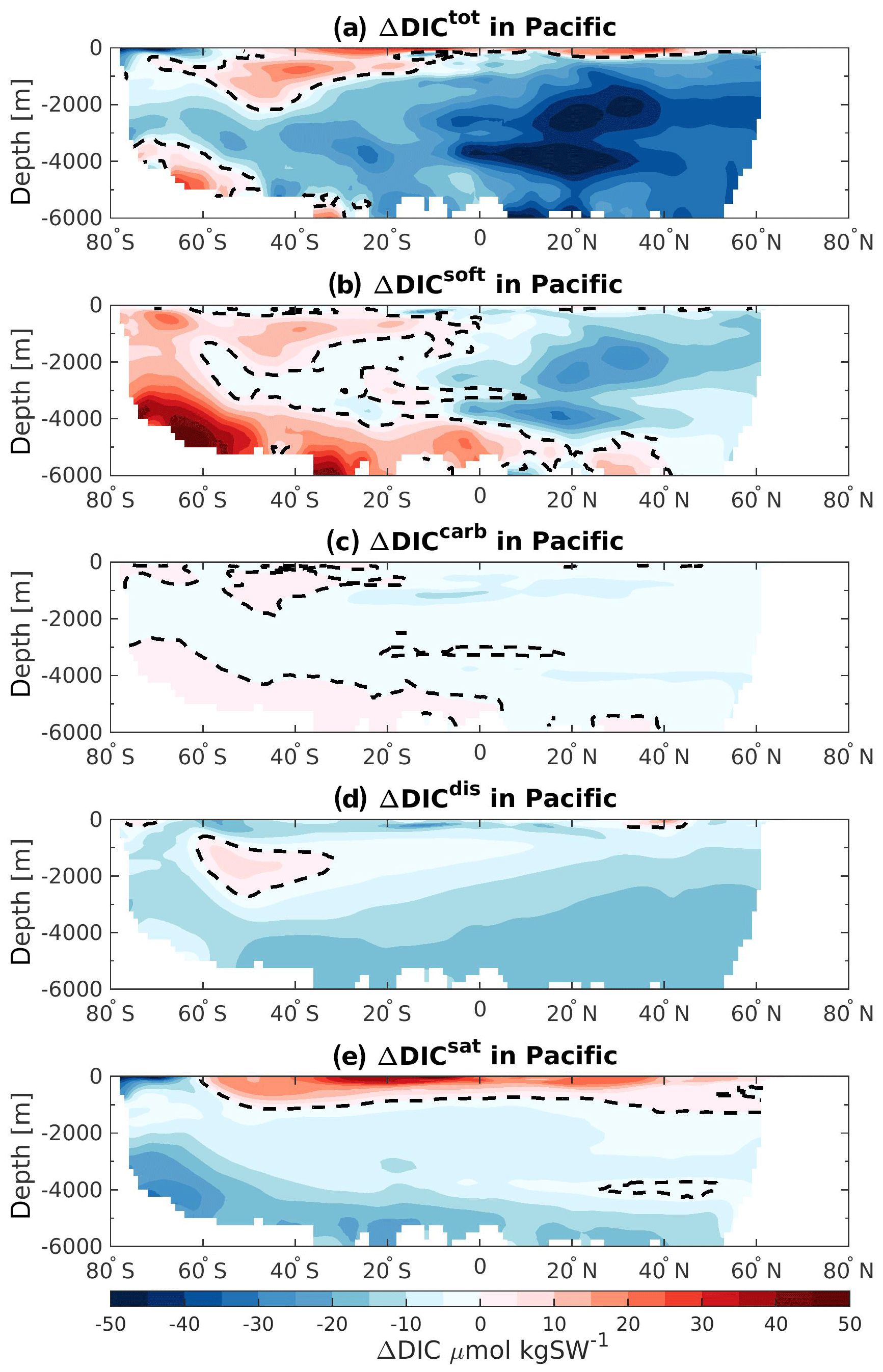
The Pacific basin shows the strongest DICtot decrease in the Northern Hemisphere, mainly due to the reduction in soft-tissue pump (Fig. 9b). This decrease in biogenic carbon is induced by a better-ventilated water mass around 30∘ N (Fig. 3c), which may come from the increase of the overturning circulation in the upper cell of the Pacific Ocean. In contrast, the DIC inventory of the high-latitude Southern Hemisphere bottom and near-surface waters is larger at 125 ka relative to 115 ka. This is attributed to the changes in soft-tissue pump, which is more effective at 125 ka due to longer residence time of the water masses (Fig. 3c). The carbonate pump has a relatively low impact on the total ΔDIC inventory in the Pacific basin but follows the same pattern as the changes in the organic carbon remineralization. The disequilibrium effect accounts for the strongest decrease of DIC throughout the basin as seen by the negative ΔDICdis in almost all regions (Fig. 9d). However, the bottom waters seem to be the most affected and become more undersaturated at 125 ka relative to 115 ka. This may be influenced by the slowing down of the subduction process in the Southern Ocean, induced by the flattening of the isopycnals. The possible higher carbon export production in the SO south of 60∘ S (Fig. 5a) may also push the water mass further out of equilibrium. Finally, the saturation component is controlling the changes occurring in the near-surface waters (Fig. 9e). Lower saturations are attributed to higher export of calcium carbonate south of 60∘ S, which lower the alkalinity at the surface and thereby the buffering capacity. On the other hand, the calcium carbonate formation decreases north of 60∘ S, resulting in a higher alkalinity and buffering capacity.
The ocean plays an important role in storing carbon and, thus, in the long term regulation of atmospheric CO2 levels. The processes involved in regulating the ocean carbon inventory are likely to change under warmer future conditions. In this study, we simulate two equilibrium states of the penultimate interglacial period using a state-of-the-art Earth system model and make a first attempt at quantifying the biogeochemical and physical processes responsible for carbon storage changes caused by different (interglacial) orbital configurations and background climates. Significant decreases in the ocean carbon storage capacity are found in a warmer climate. More than 48 % of this decrease is induced by the reduction of the biological pump. This decrease is found to be mainly driven by the shorter residence time of interior deep water masses arising from changes in Southern Ocean sea ice extent that influence the NSW and SSW mass geometry, in addition to changes in overturning circulation in the Atlantic (deeper but almost equally vigorous) and Pacific (stronger upper cell) basins.
Using the available proxy reconstructions during the LIG period allows us to assess the validity of important features in our model results. We assess the validity of the simulated 115–125 ka water mass geometry change using LIG proxy reconstructions of bottom-water δ13C, a water mass tracer strongly but inversely related to carbon and PO4 contents (Eide et al., 2017). Similar to our results, expanded SSW in the late compared to early LIG is inferred from such reconstructions to explain bottom-water δ13C decreases in different regions proximal to the Southern Ocean (Govin et al., 2009; Ninnemann and Charles, 2002). Bottom-water δ13C reconstructions indicate less influence of NSW in the deep South Atlantic at 115 ka than at 125 ka (Govin et al., 2009; Ninnemann et al., 1999). In addition, persistent (millennial-scale) mid-depth NSW ventilation extending from the LIG and into the subsequent glacial inception is also suggested based on proxy reconstructions (McManus et al., 2002; Mokeddem et al., 2014) and is consistent with model simulations (Born et al., 2011; Wang and Mysak, 2002). In our study, even though the AMOC is simulated slightly stronger and deeper at 125 ka, vigorous AMOC persists until 115 ka, ventilating the North Atlantic mid-depth. We also note that our model may not properly represent North Atlantic overflows due to its sparse resolution. This can further add uncertainties to North Atlantic water ventilation.
Also consistent with our results, ice core proxies indicate that Southern Ocean sea ice extent is greater at 115 ka than at 125 ka (Röthlisberger et al., 2008; Wolff et al., 2006), while our model reproduces the volumetric SSW expansion in response to this increase in Southern Ocean sea ice extent as suggested for glacial climates (e.g., Ferrari et al., 2014). Our model results suggest that similar sea ice (Fig. 1) and SSW expansions (Fig. 4a), albeit muted compared to glacial changes, occurred in response to LIG orbital configuration changes and without continental ice sheet growth (not included in the model), indicating a relatively tight coupling between Antarctic climate, sea ice, and the deep Atlantic water mass geometry changes influencing ocean carbon storage.
The changes in ocean carbon storage simulated by our model are significant and demonstrate that warm (interglacial) ocean carbon content changes with climate forcing. While atmospheric CO2 is fixed in our model, preventing a direct assessment of ocean carbon changes in atmospheric CO2, the decrease in deep carbon storage and shoaling of the DIC pool during the warm 125 ka interval is generally consistent with higher atmospheric CO2 levels at this time. Our estimated changes in ocean carbon budget are in the range of previous modeling studies that also suggest weaker ocean carbon storage during the beginning of the LIG (125 ka) relative to the glacial inception (115 ka). Schurgers et al. (2006) obtain a difference in atmospheric and terrestrial carbon storage of about 40 and 350 PgC, respectively, between the onset and end of the LIG. This potentially translates to a weaker ocean carbon storage of 310 PgC at the onset compared to the late LIG, which corresponds well in absolute magnitude with our findings of 314.1 PgC decrease at 125 ka. However, their simulated atmospheric CO2 steadily increases over this period, which potentially points toward more carbon needing to be stored in land or ocean toward the end of the LIG.
In contrast, Brovkin et al. (2016) simulate more ocean DICtot at 125 ka than 115 ka using simpler EMIC models. This increase is mainly attributed to the shallow-water carbonate precipitation implemented in their model. This process is not included in our model and could explain the differences in the results. However, their simulated change in atmospheric CO2 after 121 ka is in the opposite direction (an increase of roughly 20 ppm) of the atmospheric trend (a decrease of roughly 3 ppm) observed in the ice core data. This suggests that either (or both) the terrestrial or the oceanic carbon reservoir does not take up enough carbon toward the end of the LIG in order to simulate a decrease in atmospheric CO2 content.
Concerning the modification in the upper-ocean productivity under warmer climatic conditions, our model study shows a heterogeneous response in phosphate availability and carbon export production especially between the Atlantic and Pacific basins. Moore et al. (2018) also highlight such a biogeochemical divide response for future projections under warmer climatic conditions. This implies that future anthropogenic CO2 forcings may have a similar impact on the biogeochemical divide to that of past forcings. Therefore, reconstructing and understanding the large-scale productivity responses to past climate forcing are critical for assessing both global and regional sensitivity of the ocean carbon dynamic to climate change.
There are limitations to our study. Factors that could influence ocean carbon storage including sea level, riverine input of nutrients, and atmospheric dust loading are all set to preindustrial levels in our simulations but may be different in the LIG. Global sea level, for example, may be as much as 6–9 m above present levels (Kopp et al., 2009). In addition, our model does not include weathering fluxes, which might influence the carbon budget on such a long timescale. Further, we compare two quasi-equilibrated states, which is unrealistic and ignores transient forcings and shorter-term variability. This may explain differences between our model results and some proxy reconstructions. For example, proxy reconstructions suggest that both NSW and SSW ventilation may have varied considerable near 125 ka (Galaasen et al., 2014; Hayes et al., 2014). The changes suggested by these studies include reductions of NSW and expansions of SSW similar to our modeled 115–125 ka equilibrium difference, albeit occurring as short-lived (centennial-scale) transient events associated with freshwater input episodes during the final phase of northern deglaciation (Galaasen et al., 2014). Our quasi-equilibrated model simulations for 115 and 125 ka also lack ice sheet and the corresponding freshwater input variability, nor do they address such shorter-term changes that could affect the ocean carbon inventory (Stocker and Schmittner, 1997). However, short-lived changes would likely have less impact on the ocean carbon inventory than the longer-term (millennial-scale) changes we address, the latter allowing all carbon system components and ocean dynamics to adjust. Thus, we still expect our model simulations to provide insight into baseline changes and redistribution of ocean DIC forced by the different LIG orbital configurations, supported by the important role of deep Atlantic water mass geometry changes coupled with its similarity to the long-term (millennial-scale) evolution inferred from proxy reconstructions.
Ongoing anthropogenic warming raises questions about the oceanic carbon sink and its efficiency under warmer climate conditions. In this study, we use the fully coupled NorESM model to simulate two quasi-equilibrium states of the Last Interglacial: one period is globally colder (115 ka) and one is globally warmer (125 ka) than today. We focus on the differences in ocean carbon cycle that occur at 125 ka in comparison to 115 ka, specifically the differences at global and basin scales. We provide a detailed description of the biogeochemical and physical processes that are responsible for the ocean carbon inventory changes under warmer climate conditions during the LIG at the temporal and spatial scales discussed here.
We find that the global ocean carbon budget decreases during the warm (125 ka) period by 314.1 PgC and is related mainly to better ventilation in the interior ocean. The Pacific Ocean has the largest reduction and accounts for 57 % of the global DIC loss. The response of the Pacific ventilation in a warmer climate shown in this study is consistent with previous studies (Menviel et al., 2014, 2015). The Indian and Atlantic basins account for 28 % and 15 %, respectively. These quantities mostly reflect basin volumes. The SSWs are revealed to play an instrumental role for the DIC changes in the interior below 1000 m depth. In these waters, the Atlantic is highlighted to be the region where the strongest DIC loss occurs per unit volume and is characterized by a stronger ventilation and a DICtot decrease of about 37 % compared to its respective value at 115 ka.
The reduced DIC budget at 125 ka occurs mostly in the interior ocean, while there is a weak increase in the top 1000 to 1500 m depths. Two factors that contribute most to the drop in the DIC budget in the interior ocean are (1) a weaker biological component from both the soft-tissue and the carbonate pumps that dominates at the depth between 1000 and 3000 m, and (2) a stronger disequilibrium effect (i.e., more negative) of DIC in the bottom waters. However, the processes affecting the disequilibrium component can arise from different factors such as changes in the physical pump, overturning circulation, or biological pump. No general process could be attributed to its variation, which seems to be regionally affected. While the SSWs seem to become more undersaturated at 125 ka, the NSWs seem to be more saturated. Further experiments with for instance fixed biological productivity or overturning circulation could help to identify the sensitivity of this component to such factors, but they remain too expensive to perform with our model.
The weakening of the biological component at depth is driven by younger water masses simulated in the interior ocean. This decrease in residence time of the water masses is caused by the strong SST modifications that affect the ventilation at 125 ka as compared to 115 ka. Higher SST, especially at high latitudes, induces strong summer sea ice retreat in the Atlantic sector of the Southern Ocean and stratification in the Pacific Ocean. In the Atlantic basin, this results in a more southerly confined SSW and southward expansion of NSW in the deep ocean. These water masses are advected by the Antarctic circumpolar current into the Indian and the western Pacific basins. The eastern Pacific Ocean is influenced by water masses coming from the Pacific sector of the Southern Ocean, with a warmer SST that hinders the ventilation and increases the residence time of the interior water masses on the eastern side of the basin.
Concerning the modification in the upper-ocean productivity under warmer climatic conditions, our model study reveals clear yet heterogeneous changes in phosphate availability and carbon export production especially between the Atlantic and Pacific basins. Such inter-basinal response in the biogeochemical divide is also highlighted by Moore et al. (2018) for future projections under warmer climatic conditions. This implies that changes in the biogeochemical divide could be somewhat similarly impacted from past and future anthropogenic CO2 forcings, although the basin-specific responses suggest that it may not be a priori simple to predict the pattern or sign of the response of large-scale productivity to a given common forcing. Given the economic importance of basin scale productivity and the sensitivity found in past and future simulations, reconstructing and understanding the pattern and validating the sign and (model) response of large scale productivity to climate forcing are therefore critical for assessing not only the sign but also the sensitivity of global productivity to climate change.
The remaining uncertainties include, among others, the use of preindustrial states for some boundary conditions and the absence of freshwater input, which could modify the spatial response, particularly during the early interglacial period, which might include the final episodes of continental deglaciation. This is due to the lack of knowledge on such forcing during past climate conditions. Additional model-based studies using different Earth system models would be useful to confirm the robustness of our finding and further improve our understanding of the carbon dynamics and the feedback in the ocean under warmer climate conditions. Finally, our model-based study suggests that past warm periods experienced considerable carbon cycle and ocean DIC changes, linked to the response of the interior-ocean ventilation and biological productivity to high-latitude warming and interglacial background climate differences. It also suggests that the Atlantic part of the Southern Ocean is most sensitive to past climate change and hence could be a potential indicator of similar large-scale circulation changes in the future. Close monitoring of this region could be critical to better understand climate feedback on the carbon cycle under future warmer climate conditions.
The model data are available on the Norwegian Research Data Archive server (https://doi.org/10.11582/2018.00038; Kessler, 2018).
AK and JP designed and analyzed the simulations, and wrote the first the first draft of the paper. EVG and USN revised and provided input on the paper. All authors discussed the results.
The authors declare no competing interests.
We thank Victor Brovkin and the two anonymous referees for their positive and
constructive comments, which helped to clarify the manuscript. We also thank
the editor, Laurie Menviel, for the time she dedicated in processing our
manuscript and for her additional comments and suggestions. We thank
Nadine Goris for her valuable feedback on the first draft of the manuscript.
We are grateful to Chuncheng Guo for his technical assistance. This work was
supported by the Research Council of Norway-funded
projects THRESHOLDS (254964) and ORGANIC (239965) and
the Bjerknes Centre for Climate Research project BIGCHANGE. We acknowledge
the Norwegian Metacenter for Computational Science and Storage Infrastructure
(Notur/Norstore) projects nn2345k, ns2345k, nn1002k, and ns1002k for
providing the computing and storing resources essential for this
study.
Edited by: Laurie Menviel
Reviewed by: Victor Brovkin and two anonymous referees
Bentsen, M., Bethke, I., Debernard, J. B., Iversen, T., Kirkevåg, A., Seland, Ø., Drange, H., Roelandt, C., Seierstad, I. A., Hoose, C., and Kristjánsson, J. E.: The Norwegian Earth System Model, NorESM1-M – Part 1: Description and basic evaluation of the physical climate, Geosci. Model Dev., 6, 687–720, https://doi.org/10.5194/gmd-6-687-2013, 2013. a
Bernadello, R., Marinov, I., Palter, J. B., Sarmiento, J. L., Galbraith, E. D., and Slater, R. D.: Response of the Ocean Natural Carbon Storage to Projected Twenty–First–Century Climate Change, J. Climate, 27, 2033–2053, https://doi.org/10.1175/JCLI-D-13-00343.1, 2014. a
Bleck, R., Rooth, C., Hu, D., and Smith, L. T.: Salinity-driven thermocline transients in a wind– and thermohaline–forced isopycnic coordinate model of the north Atlantic, J. Pys. Oceanogr., 22, 1486–1505, https://doi.org/10.1175/1520-0485(1992)022<1486:SDTTIA>2.0.CO;2, 1992. a, b
Born, A., Nisancioglu, K. H., and Risebrobakken, B.: Late Eemian warming in the Nordic Seas as seen in proxy data and climate models, Paleoceanography, 26, PA2207, https://doi.org/10.1073/pnas.1322103111, 2011. a
Broecker, W. S.: ”NO”, A conservative water-mass tracer, Earth Planet. Sc. Lett., 23, 100–107, https://doi.org/10.1016/0012-821X(74)90036-3, 1974. a, b
Brovkin, V., Brücher, T., Kleinen, T., Zaehle, S., Joos, F., Roth, R., Spahni, R., Schmitt, J., Fischer, H., Leuenberger, M., Stone, E. J., Ridgwell, A., Chapellaz, J., Kehrwald, N., Barbante, C., Blunier, T., and Jensen, D. D.: Comparative carbon cycle dynamics of the present and last interglacial, Quaternary Sci. Rev., 137, 15–32, https://doi.org/10.1016/j.quascirev.2016.01.028, 2016. a, b
Capron, E., Govin, A., Stone, E. J., Masson-Delmotte, V., Mulitza, S., Otto-Bliesner, B., Rasmussen, T. L., Sime, L. C., Waelbroeck, C., and Wolff, E. W.: Temporal and spatial structure of multi-millennial temperature changes at high latitudes during the Last Interglacial, J. Quaternary Sci., 103, 116–133, https://doi.org/10.1016/j.quascirev.2014.08.018, 2014. a
Dickson, A. G. and Millero, F. J.: A comparison of the equilibrium constants for the dissociation of carbonic acid in seawater media, Deep-Sea Res., 34, 1733–1743, https://doi.org/10.1016/0198-0149(87)90021-5, 1987. a
Dorthe Dahl-Jensen, Gogineni, P., and White, J. W. C.: Reconstruction of the last interglacial period from the NEEM ice core, Nature, 493, 489–489, 2013. a
Duteil, O., Koeve, W., Oschlies, A., Aumont, O., Bianchi, D., Bopp, L., Galbraith, E., Matear, R., Moore, J. K., Sarmiento, J. L., and Segschneider, J.: Preformed and regenerated phosphate in ocean general circulation models: can right total concentrations be wrong?, Biogeosciences, 9, 1797–1807, https://doi.org/10.5194/bg-9-1797-2012, 2012. a
Eide, M., Olsen, A., Ninnemann, U. S., and Johannessen, T.: A global ocean climatology of preindustrial and modern ocean δ13C, Global Biogeochem. Cy., 31, 515–534, https://doi.org/10.1002/2016GB005473, 2017. a
Eppley, R. W.: Temperature and phytoplankton growth in the sea, Fish. B.-NOAA, 70, 1063–1085, 1972. a
Ferrari, R., Jansen, M. F., Adkins, J. F., Burke, A., Stewart, A. L., and Thompson, A. F.: Antarctic sea ice control on ocean circulation in present and glacial climates, P. Natl. Acad. Sci. USA, 111, 8753–8758, https://doi.org/10.1073/pnas.1323922111, 2014. a, b
Follows, M. and Williams, R.: Mechanisms controlling the air–sea flux of CO2 in the North Atlantic, The Ocean Carbon Cycle and Climate, edited by: Follows, M. and Oguz, T., Kluwer Academic, 217–249, https://doi.org/10.1007/978-1-4020-2087-2_7, 2004. a
Galaasen, E. V., Ninnemann, U. S., Irvali, N., Kleiven, H. F., Rosenthal, Y., Kissel, C., and Hodell, D. A.: Rapid Reductions in North Atlantic Deep Water During the Peak of the Last Interglacial Period, Science, 343, 1129–1132, https://doi.org/10.1126/science.1248667, 2014. a, b
Govin, A., Michel, E., Labeyrie, L., Waelbroeck, C., Dewilde, F., and Jansen, E.: Evidence for northward expansion of Antarctic Bottom Water mass in the Southern Ocean during the last glacial inception, Paleoceanography, 24, PA1202, https://doi.org/10.1029/2008PA001603, 2009. a, b, c
Gu, D. and Philander, S. G. H.: Interdecadal climate fluctuations that depend on exchanges between the tropics and extratropics, Science, 275, 805–807, https://doi.org/10.1126/science.275.5301.805, 1997. a
Guo, C., Bentsen, M., Bethke, I., Ilicak, M., Tjiputra, J., Toniazzo, T., Schwinger, J., and Otterå, O. H.: Description and evaluation of NorESM1-F: A fast version of the Norwegian Earth System Model (NorESM), Geosci. Model Dev. Discuss., https://doi.org/10.5194/gmd-2018-217, in review, 2018. a
Hayes, C. T., Martinez-Garcia, A., Hasenfratz, A., Jaccard, S. L., Hodell, D. A., Sigman, D. M., Haug, G. H., and Anderson, R. F.: A stagnation event in the deep South Atlantic during the last interglacial period, Science, 346, 1514–1517, https://doi.org/10.1126/science.1256620, 2014. a
Heinze, C., Maier-Reimer, E., Winguth, A. M. E., and Archer, D.: A global oceanic sediment model for long-term climate studies, Global Biogeochem. Cy., 13, 221–250, https://doi.org/10.1029/98GB02812, 1999. a
Hoffman, J. S., Clark, P. U., Parnell, A. C., and He, F.: Regional and global sea-surface temperatures during the last interglaciation, Science, 355, 276–279, https://doi.org/10.1126/science.aai8464, 2017. a, b
Kessler, A.: NorESM-F_LIG115_LIG125_year_4951-5000 [Data set], Norstore, https://doi.org/10.11582/2018.00038, 2018. a, b
Kleinen, T., Brovkin, V., and Munhoven, G.: Modelled interglacial carbon cycle dynamics during the Holocene, the Eemian and Marine Isotope Stage (MIS) 11, Clim. Past, 12, 2145–2160, https://doi.org/10.5194/cp-12-2145-2016, 2016. a
Kopp, R. E., Simons, F. J., Mitrovica, J. X., Maloof, A. C., and Oppenheimer, M.: Probabilistic assessment of sea level during the last interglacial stage, Nature, 462, 863–867, https://doi.org/10.1038/nature08686, 2009. a
Lawrence, D. M., Oleson, K. W., Flanner, M. G., Fletcher, C. G., Lawrence, P. J., Levis, S., Swenson, S. C., and Bonan, G. B.: The CCSM4 land simulation, 1850–2005: assessment of surface climate and new capabilities, J. Climate, 25, 2240–2260, https://doi.org/10.1175/JCLI-D-11-00103.1, 2012a. a
Lourantou, A., Chappellaz, J., Barnola, J. M., Masson-Delmotte, V., and Raynaud, D.: Changes in atmospheric CO2 and its carbon isotopic ratio during the penultimate deglaciation, Quaternary Sci. Rev., 29, 1983–1992, https://doi.org/10.1016/j.quascirev.2010.05.002, 2010. a
Luo, Y., Tjiputra, J. F., Guo, C., Zhang, Z., and Lippold, J.: Atlantic deep water circulation during the last interglacial, Sci. Rep.-UK, 8, 4401, https://doi.org/10.1038/s41598-018-22534-z, 2018. a, b, c, d
Maier-Reimer, E.: Geochemical cycles in an ocean general circulation model, preindustrial tracer distributions, Global Biogeochem. Cy., 7, 645–677, https://doi.org/10.1029/93GB01355, 1993. a
Maier-Reimer, E., Kriest, I., Segschneider, J., and Wetzel, P.: The HAMburg Ocean Carbon Cycle Model HAMOCC5.1 – Technical Description Release 1.1, Berichte zur Erdsystemforschung 14, ISSN 1614-1199, Max Planck Institute for Meteorology, Hamburg, Germany, 50 pp., 2005. a, b
Marinov, I., Gnanadesikan, A., Toggweiler, R., and Sarmiento, J. L.: The Southern Ocean Biogeochemical Divide, Nature, 441, 946–967, https://doi.org/10.1038/nature04883, 2006. a
Masson-Delmotte, V., Stenni, B., Pol, K., Braconnot, P., Cattani, O., Falourd, S., Kageyama, M., Jouzel, J., Landais, A., Minster, B., Barnola, J. M., Chappellaz, J., Krinner, G., Johnsen, S., Röthlisberger, R., Hansen, J., Mikolajewicz, U., and Otto-Bliesner, B.: EPICA Dome C record of glacial and interglacial intensities, Quaternary Sci. Rev., 29, 113–128, https://doi.org/10.1016/j.quascirev.2009.09.030, 2010. a
McManus, J. F., Oppo, D. W., Keigwin, L. D., Cullen, J. L., and Bond, G. C.: Thermohaline circulation and prolonged interglacial warmth in the North Atlantic, Quaternary Res., 58, 17–21, https://doi.org/10.1006/qres.2002.2367, 2002. a, b
Mehrbach, C., Culberson, C. H., Hawley, J. E., and Pytkwicz, R. M.: Measurement of the apparent dissociation constants of carbonic acid in seawater at atmospheric pressure, Limnol. Oceanogr., 18, 897–907, https://doi.org/10.4319/lo.1973.18.6.0897, 1973. a
Menviel, L., Joos, F., and Ritz, S. P.: Simulating atmospheric CO2, δ13C and the marine carbon cycle during the Last Glaciale/Interglacial cycle: possible role for a deepening of the mean remineralization depth and an increase in the oceanic nutrient inventory, Quaternary Sci. Rev., 56, 46–68, https://doi.org/10.1016/j.quascirev.2012.09.012, 2012. a
Menviel, L., England, M. H., Meissner, K. J., Mouchet, A., and Yu, J.: Atlantic-Pacific seesaw and its role in outgassing CO2 during Heinrich events, Paleoceanography, 29, 58–70, https://doi.org/10.1002/2013PA002542, 2014. a
Menviel, L., Mouchet, A., Meissner, K. J., Joos, F., and England, M. H.: Impact of oceanic circulation changes on atmospheric δ13CO2, Global Biogeochem. Cy., 29, 1944–1961, https://doi.org/10.1002/2015GB005207, 2015. a
Mokeddem, Z., McManus, J. F., and Oppo, D. W.: Oceanographic dynamics and the end of the last interglacial in the subpolar North Atlantic, P. Natl. Acad. Sci. USA, 111, 11253–11268, https://doi.org/10.1073/pnas.1322103111, 2014. a, b
Moore, J. K., Fu, W., Primeau, F., Britten, G. L., Lindsay, K., Long, M., Doney, S. C., Mahowald, N., Hoffman, F., and Randerson, J. T.: Sustained climate warming drives declining marine biological productivity, Science, 359, 1139–1143, https://doi.org/10.1126/science.aao6379, 2018. a, b, c, d
Ninnemann, U. S. and Charles, C. D.: Changes in the mode of Southern Ocean circulation over the last glacial cycle revealed by foraminiferal stable isotopic variability, Earth Planet. Sc. Lett., 201, 383–396, https://doi.org/10.1016/S0012-821X(02)00708-2, 2002. a
Ninnemann, U. S., Charles, C. D., and Hodell, D. A.: Origin of global millennial scale climate events: constraints from the Southern Ocean deep sea sedimentary record, Geophysical Monograph-American Geophysical Union, 112, 99–112, 1999. a
Otto-Bliesner, B. L., Marshall, S. J., Overpeck, J. T., Miller, G. H., Hu, A., and CAPE Last Interglacial Project members: Simulating Arctic Climate Warmth and Icefield Retreat in the Last Interglaciation, Science, 311, 1751–1753, https://doi.org/10.1126/science.1120808, 2006. a
Otto-Bliesner, B., Rosenbloom, N., Stone, E., Mckay, N. P., Lunt, D. J., Brady, E. C., and Overpeck, J. T.: How warm was the Last Interglacial? New model-data comparisons, Philos. T. R. Soc. A, 371, 20130097, https://doi.org/10.1098/rsta.2013.0097, 2013. a
Ridgwell, A.: Glaciale/Interglacial Perturbations in the Global Carbon Cycle, PhD thesis, University of East Anglia, Norwich, UK, 2001. a
Röthlisberger, R., Mudelsee, M., Bigler, M., de Angelis, M., Fischer, H., Hansson, M., Lambert, F., Masson-Delmotte, V., Sime, L., Udisti, R., and Wolff, E. W.: The Southern Hemisphere at glacial terminations: insights from the Dome C ice core, Clim. Past, 4, 345–356, https://doi.org/10.5194/cp-4-345-2008, 2008. a
Sarmiento, J. L., Slater, R., Barber, R., Bopp, L., Doney, S. C., Hirst, A. C., Kleypas, J., Matear, R., Mikolajewicz, U., Monfray, P., Soldatov, V., Spall, S. A., and Stouffer, R.: Response of ocean ecosystems to climate warming, Global Biogeochem. Cy., 18, GB3003, https://doi.org/10.1029/2003GB002134, 2004a. a
Sarmiento, J. L., Gruber N., Brzezinski, M. A., and Dunne, J. P.: High-latitude controls of thermocline nutrients and low latitude biological productivity, Nature, 427, 56–60, https://doi.org/10.1038/nature02127, 2004b. a
Schneider, R., Schmitt, J., Köhler, P., Joos, F., and Fischer, H.: A reconstruction of atmospheric carbon dioxide and its stable carbon isotopic composition from the penultimate glacial maximum to the last glacial inception, Clim. Past, 9, 2507–2523, https://doi.org/10.5194/cp-9-2507-2013, 2013. a
Schurgers, G., Mikolajewicz, U., Gröger, M., Maier-Reimer, E., Vizcaíno, M., and Winguth, A.: Dynamics of the terrestrial biosphere, climate and atmospheric CO2 concentration during interglacials: a comparison between Eemian and Holocene, Clim. Past, 2, 205–220, https://doi.org/10.5194/cp-2-205-2006, 2006. a, b
Sigman, D. and Boyle, E.: Glacial/interglacial variations in atmospheric carbon dioxide, Nature, 407, 859–869, https://doi.org/10.1038/35038000, 2000. a
Smith, E. L.: Photosynthesis in relation to light and carbon dioxide, P. Natl. Acad. Sci. USA, 22, 504–511, 1936. a
Stocker, T. F. and Schmittner, A.: Influence of CO2 emission rates on the stability of the thermohaline circulation, Nature, 388, 862–865, https://doi.org/10.1038/42224, 1997. a
Tjiputra, J. F., Roelandt, C., Bentsen, M., Lawrence, D. M., Lorentzen, T., Schwinger, J., Seland, Ø., and Heinze, C.: Evaluation of the carbon cycle components in the Norwegian Earth System Model (NorESM), Geosci. Model Dev., 6, 301–325, https://doi.org/10.5194/gmd-6-301-2013, 2013. a
Turney, C. S. M. and Jones, R. T.: Does the Agulhas Current amplify global temperatures during super-interglacials?, J. Quaternary Sci., 25, 839–843, https://doi.org/10.1002/jqs.1423, 2010. a
van Heuven, S., Pierrot, D., Rae, J. W. B., Lewis, E., and Wallace, D. W. R.: Matlab program developed for CO2 system calculations. ornl/cdiac-105b., Carbon Dioxide Information Analysis Center, Oak Ridge National Laboratory, US Department of Energy, Oak Ridge, Tennessee, available at: http://cdiac.ornl.gov/ftp/co2sys/CO2SYS_calc_MATLAB_v1.1/ (last access: 5 December 2018), 2011. a
Wang Z. and Mysak, L. A.: Simulation of the last glacial inception and rapid ice sheet growth in the McGill Paleoclimate Model, Geophys. Res. Lett., 29, 2102, https://doi.org/10.1029/2002GL015120, 2002. a
Wanninkhof, R.: Relationship between wind speed and gas exchange over the ocean, J. Geophys. Res., 97, 7373–7382, https://doi.org/10.1029/92JC00188, 1992. a
Weiss, R. F.: The solubility of nitrogen, oxygen and argon in water and sea water, Deep-Sea Res., 17, 721–735, https://doi.org/10.1016/0011-7471(70)90037-9, 1970. a
Weiss, R. F.: Carbon dioxide in water and seawater: the solubility of a non–ideal gas, Mar. Chem., 2, 203–215, https://doi.org/10.1016/0304-4203(74)90015-2, 1974. a
Wolff, E. W., Fischer, H., Fundel, F., Ruth, U., Twarloh, B., Littot, G. C., Mulvaney, R., Röthlisberger, R., de Angelis, M., Boutron, C. F., Hansson, M., Jonsell, U., Hutterli, M. A., Lambert, F., Kaufmann, P., Stauffer, B., Stocker, T. F., Steffensen, J. P., Bigler, M., Siggaard-Andersen, M. L., Udisti, R., Becagli, S., Castellano, E., Severi, M., Wagenbach, D., Barbante, C., Gabrielli P., and Gaspari, V.: Southern Ocean sea-ice extent, productivity and iron flux over the past eight glacial cycles, Nature, 440, 491–496, https://doi.org/10.1038/nature04614, 2006. a