Generalized Extreme Value Statistics, Physical Scaling and Forecasts of Oil Production in the Bakken Shale


The Ali I. Al-Naimi Petroleum Engineering Research Center, King Abdullah University of Science and Technology, Thuwal 23955-6900, Saudi Arabia
*
Author to whom correspondence should be addressed.
Energies 2019, 12(19), 3641; https://doi.org/10.3390/en12193641
Submission received: 18 August 2019
/
Revised: 10 September 2019
/
Accepted: 16 September 2019
/
Published: 24 September 2019
(This article belongs to the Special Issue Improved Reservoir Models and Production Forecasting Techniques for Multi-Stage Fractured Hydrocarbon Wells)
Abstract
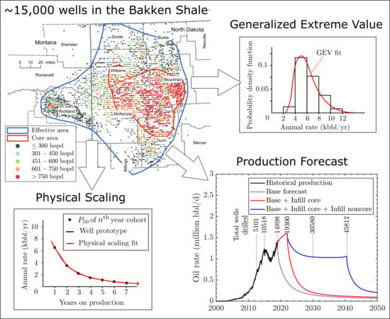
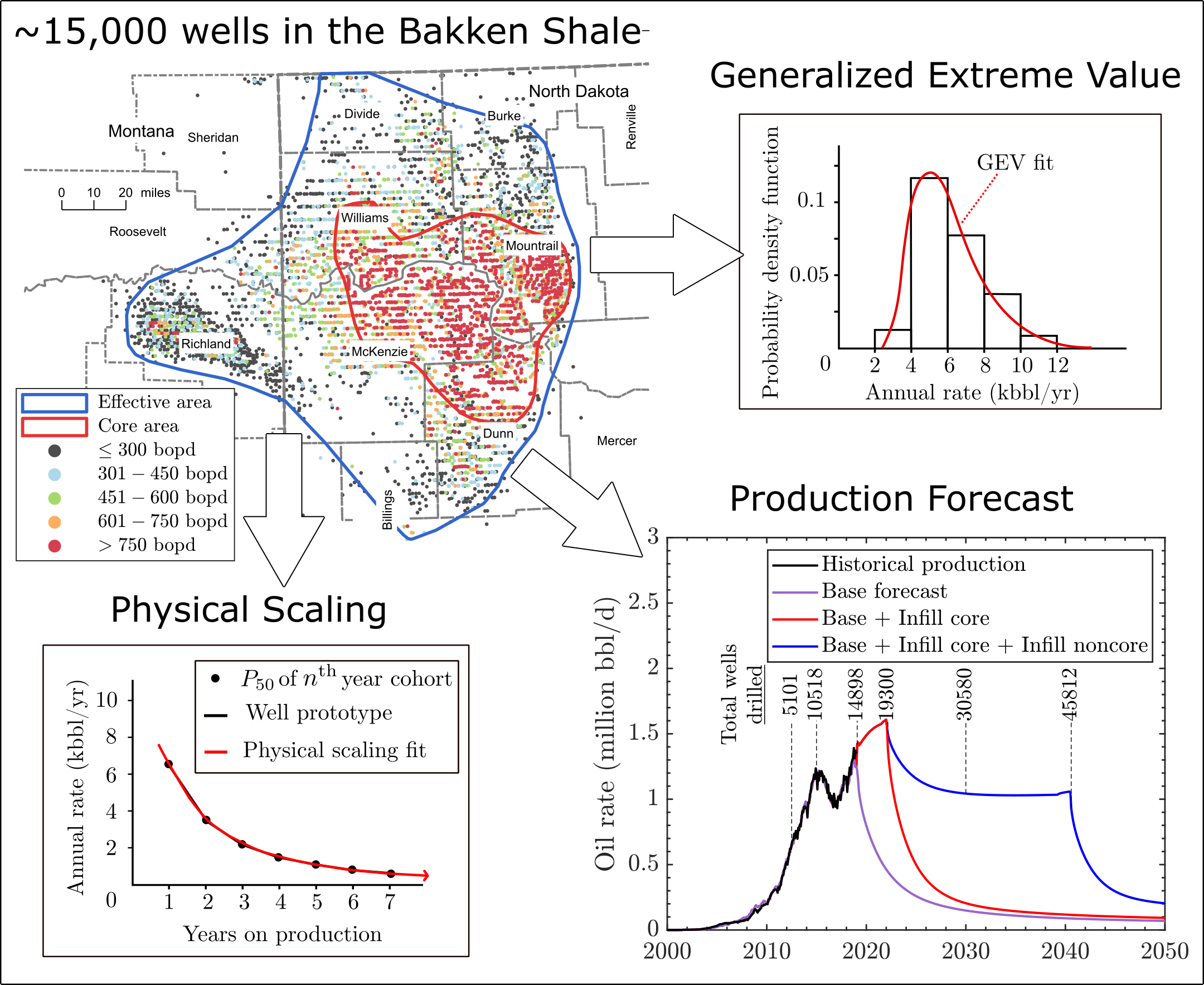
:We aim to replace the current industry-standard empirical forecasts of oil production from hydrofractured horizontal wells in shales with a statistically and physically robust, accurate and precise method of matching historic well performance and predicting well production for up to two more decades. Our Bakken oil forecasting method extends the previous work on predicting fieldwide gas production in the Barnett shale and merges it with our new scaling of oil production in the Bakken. We first divide the existing 14,678 horizontal oil wells in the Bakken into 12 static samples in which reservoir quality and completion technologies are similar. For each sample, we use a purely data-driven non-parametric approach to arrive at an appropriate generalized extreme value (GEV) distribution of oil production from that sample’s dynamic well cohorts with at least years on production. From these well cohorts, we stitch together the , , and statistical well prototypes for each sample. These statistical well prototypes are conditioned by well attrition, hydrofracture deterioration, pressure interference, well interference, progress in technology, and so forth. So far, there has been no physical scaling. Now we fit the parameters of our physical scaling model to the statistical well prototypes, and obtain a smooth extrapolation of oil production that is mechanistic, and not just a decline curve. At late times, we add radial inflow from the outside. By calculating the number of potential wells per square mile of each Bakken region (core and noncore), and scheduling future drilling programs, we stack up the extended well prototypes to obtain the plausible forecasts of oil production in the Bakken. We predict that Bakken will ultimately produce 5 billion barrels of oil from the existing wells, with the possible addition of 2 and 6 billion barrels from core and noncore areas, respectively.
1. Introduction
Over the last decade, crude oil and gas production from hydrofractured shales in the United States has accounted for most of the net increase of global crude oil production. Therefore, it is important to have a reliable, quantitative method for delineating the possible futures oil and gas production in the data-rich US shales. The current industry-standard methods of forecasting production from shales are variants of the empirical decline curve analysis (DCA) [1], developed 75 years ago. Lately, some of the more sophisticated methods, for example, Fractional Decline Curve [2] have become popular.
Unlike other analytical and numerical methods that require numerous reservoir parameters and a lengthy calculation or simulation time, DCA only requires production data to predict future production by extrapolating oil or gas rate observed in a boundary-dominated flow regime. Because of DCA’s simplicity, most petroleum engineers adopt it for reserve assessment in shales, including Estimated Ultimate Recovery (EUR) predictions from USGS [3,4] and EIA [5].
USGS first split the Bakken region into 6 assessment units (AUs) and defined sweet spots. Then, they calculated the number of wells that could be drilled in each AU by dividing its total area with the average drainage area per well. In parallel, they used DCA to calculate the average EURs for sweet spots and other areas. The 7.4 billion barrels of undiscovered technically recoverable oil was obtained by multiplying the total number of wells that could be drilled in each AU with the corresponding average EUR multiplied by the untested fraction of that AU. EIA used a similar approach by dividing the Bakken region into 5 AUs and refining them by counties to determine the infill well potential. Both USGS and EIA predictions were assessed by Hughes [6,7,8,9]. We predict that the undiscovered, technically recoverable oil in the Bakken is 2 billion bbls in the core area and it might be 6 billion bbls in the noncore area (Figure 1) or 8 billion barrels in total.
Most shale wells do not reach the boundary-dominated flow regime for their entire production lives because of the vanishing matrix permeability. Thus, the traditional DCA frequently overestimates EURs of shale wells. To address this issue, many authors have suggested improved DCA methods, specific to shale wells: the Power Law Exponential Decline [10], the Stretched Exponential Decline [11], the Logistic Growth Model [12], the Extended Exponential DCA [13], and the Extended Hyperbolic DCA [14]. To make things worse, the empirical DCA fits of particular wells are ill-suited to forecasting production from a wide area of a given shale play in which reservoir properties vary and uncertainties abound. Therefore, some authors have developed probabilistic models to introduce a range of possible outcomes into their production forecasts [15,16,17,18,19,20]. The most common assumption is that well productivities in shales are log-normally distributed.
In this paper, we adopt a hybrid data-driven and physics-based method of predicting oil or gas production in shales that has been introduced in our previous work [21,22]. Here, we consider only black oil production. First, we identify play regions in which reservoir quality is similar, see Figure 1. In each region, we identify well classes by different completion technologies. Finally, a well class in a region constitutes a well sample. We ensure that oil production from all wells in each sample is statistically uniform, that is, has a unimodal distribution. For each well sample, we then identify well cohorts with at least years on production. In general, well cohorts contain different sets of wells that satisfy the minimum time on production required for each cohort. It turns out that each cohort of wells is superbly characterized by its unique Generalized Extreme Value (GEV) distribution (see Appendix A) of annualized well rates or cumulative well production. Different cohorts in the same sample have different GEV distributions, each with its unique expected value, median and mode. Here we choose the somewhat better GEV fits of the production rate distributions. Each GEV distribution is statistically superior to the corresponding log-normal distribution at the 95% confidence level. When we plot the expected values of the GEV distributions of all wells cohorts in a sample versus elapsed time of production, we obtain this sample’s average statistical well prototype that is purely field data-driven.
Now we fit each statistical well prototype with a physical scaling curve that extends this prototype to 30 years on production. The physical scaling curves are based on an analytical solution of the pressure diffusion equation in the hydrofractured horizontal shale well geometry. In previous papers, we comprehensively detailed the physical scaling solutions for shale gas wells [23,24] and shale oil wells [22,25]. Late-time flow from outer reservoir encompassing the stimulated reservoir volume (SRV) [26] was also quantified. We have verified that our physical scaling is equivalent to detailed numerical reservoir simulations [27]. This scaling is much simpler to set up and runs almost infinitely faster than the corresponding reservoir simulations.
At this point, for each well sample in every play region, we have obtained a unique hybrid mean () well prototype with 30 years on production. In each play region, we know how many wells were drilled and completed each month up until current time. We then multiply each well prototype by the number of wells completed per month and stack them up to represent the total historical field rate and future production decline. In this manner, we obtain a ‘base’ case forecast for all existing wells. This base case forecast is a ‘do nothing’ scenario with no new wells drilled in the future. For all other forecasts of future field production rate, we first determine the infill potential or the number of wells that can be drilled in the future without causing significant interwell pressure interference (fracture hits). We cover each region with a fish-net grid that consists of one-square-mile pixels. We then calculate the infill potential as the number of wells that can be drilled so that the total number of wells in each pixel is less than the maximum allowable number of wells without fracture hits. Next, based on the infill potentials for all regions, we create future drilling programs to obtain plausible forecasts of oil or gas production. Based on current rig count in the Bakken, we assume a constant overall drilling rate. Finally, we assign the correct well prototype to every future well that will be drilled during each month of a postulated drilling schedule, and sum them up to obtain a forecast scenario.
In this paper, we select the Bakken shale, the current second-largest oil producer in the U.S. with 1.5 million bbl of oil per day, as an illustration. Being one of the oldest shale oil plays, Bakken has been a field laboratory to test drilling and completion technologies and increase well productivity. Currently, Bakken has ∼15,000 active hydrofractured horizontal wells with a few wells that have 18 years of production data. In a previous paper [22], we scaled well-by-well all ∼15,000 wells in the Bakken. We accounted for well refracturing and/or changes in downhole pressure. It turns out that the 12 well prototypes obtained with our hybrid GEV–physical scaling method are as good in duplicating the total field rate as the super-precise scaling of each individual well in our previous work [22]. Given the results of our analyses that are free of bias, policy-makers should not assume that the production boom in the Bakken shale will last decades longer.
2. Results
Our approach is as follows:
- Divide all 14,678 horizontal oil wells in the Bakken shale into 12 samples in which oil production is statistically uniform;
- Fit a generalized extreme value distribution to all wells in every sample and obtain 12 stable mean well prototypes;
- Fit the physics-based scaling curves to every statistical well prototype and extend these prototypes smoothly to 30 years on production;
- Replace oil production from all existing wells with the 12 extended well prototypes and obtain a ‘base’ forecast;
- Calculate the infill potential for each of the 12 regions in the Bakken; and
- Create the plausible infill drilling schedules and forecast total field oil production rate up to the year 2050.
2.1. Design of Well Regions
In the previous work [21], we divided all 13,141 horizontal wells in the Barnett shale into 6 static regions that corresponded to the geographical borders of 6 major gas-producing counties. We justified this approach as follows: (i) Productive Barnett shale is a single gas reservoir; (ii) the Barnett play area is relatively small, and the division into counties captures different reservoir qualities; and (iii) completion technologies have not been revolutionized over time.
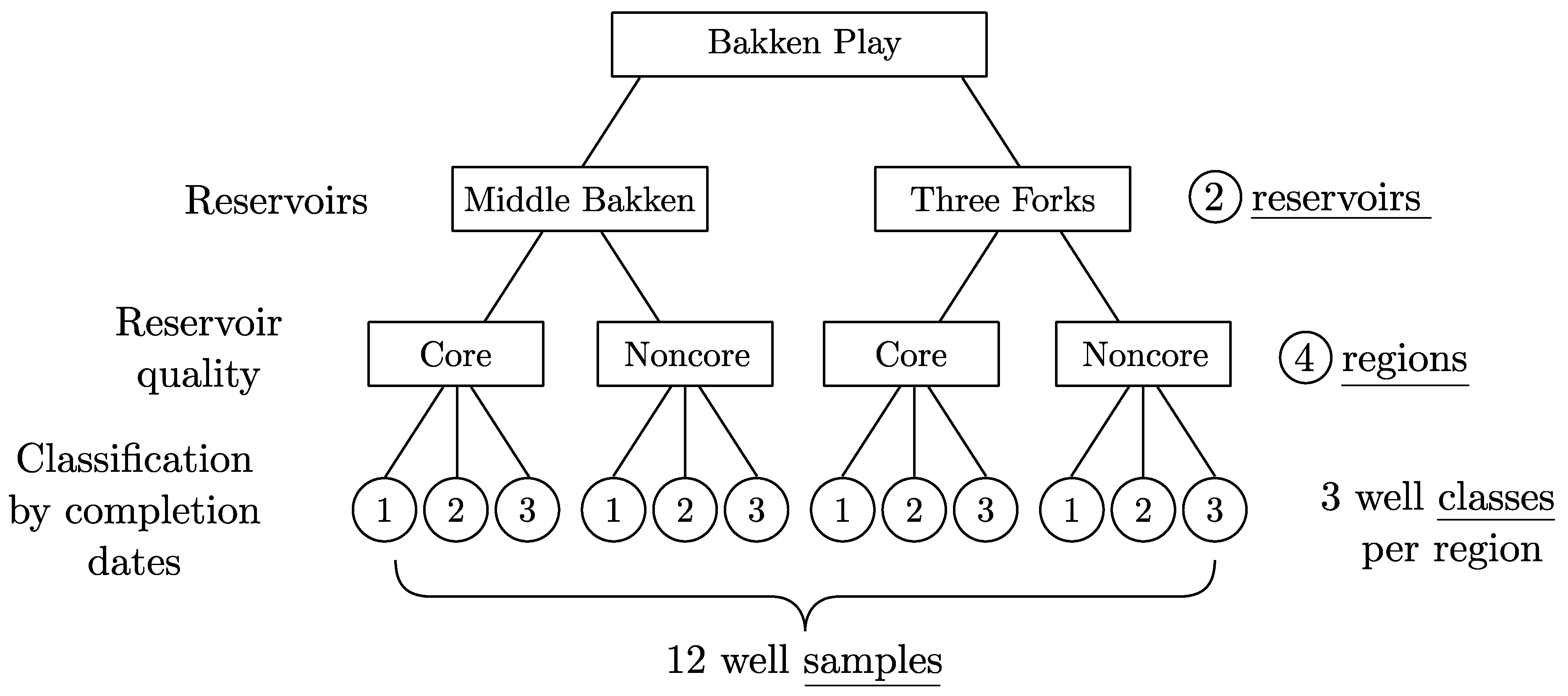
However, in the Bakken shale, we introduce a more complicated set of 12 static well samples classified by reservoir, geography, and completion dates. In Bakken, there are two different producing reservoirs, the Middle Bakken and Three Forks. Accordingly, we first split all Bakken wells into the Middle Bakken and Three Forks groups. To account for different reservoir quality, we then divide each of these two well groups into two macro regions: the core and noncore areas, see Figure 2. Finally, we further refine the four Bakken macro regions by splitting them into three classes by completion date intervals, 2000–2012, 2013–2016 and 2017–2019. These classes reflect advancements in well completion technology, such as longer wells, more fracture stages, fewer clusters and perforation shots, bigger hydrofractures, more proppant, and so forth. In the end, we divide the existing 14,678 horizontal oil wells in the Bakken into 12 unique samples listed in Table 1.
2.2. Statistical Well Prototypes
For each of the 12 Bakken well samples defined in Section 2.1, we construct a statistical well prototype based on the Generalized Extreme Value (GEV, see Appendix A) mean or the values of annual rates from all well cohorts that exist in that particular region. Figure 3 illustrates the procedure of arriving at the GEV well prototypes. For every GEV distribution fit we acquire values of the location parameter (), scale parameter (), shape parameter (), confidence interval (CI), mean (), median, mode, and . In this paper, we show only two GEV fit examples (Figure 4 and Figure 5). Please see Supporting Online Materials-1 to find all GEV fits for all 12 regions of the Bakken shale. The resulting statistical well prototypes are plotted versus the square root of time on production in Figure 6. In the initial year on production, for some well cohorts, time was shifted by subtracting the first 1–3 months on production (see the second column of Table 2) to discount all possible initial disturbances in well performance. After these time shifts, each mean or well prototype starts from a straight line versus the square root of time on production, as expected in linear flow regime. Later, cumulative oil production bends down due to the inter-hydrofracture pressure interference and exponential decline of production rate [23]. For our GEV distribution fits, the mean or prototype is always higher than the median, and the median is higher than the mode. The and prototypes diverge from the mean with time, indicating that with time the best wells grow better and worst wells worse. A similar trend was also observed in the Barnett shale [21].
2.3. Physical Scaling Fits
For each region, we fit the statistical well prototype with a physical scaling curve, see Appendix B, to extend this prototype to 30 years on production. The fitting procedure is detailed in the Materials and Methods section. Briefly, by least squares fit, we find optimum values of the scaling parameters and so that the physics-based well prototypes match the statistical well prototypes. The results are shown in Figure 6. The red solid lines show the most pessimistic versions of each physics-based prototype, which assume that oil is produced only from the interior of the stimulated reservoir volume (SRV). The green solid lines show a more realistic forecast with an assumption that at late times there will be additional exterior flow of towards the SRV. Finally, one obtains the Estimated Ultimate Recovery (EUR) from each region by identifying the endpoint of cumulative production for the physics-scaling prototype. In Table 2, the scaling parameters, , and a, and EUR values are listed for each region with and without exterior flow. Notice that in general the newest wells have the shortest pressure interference times, , and fastest decline rates.
2.4. Base or ‘Do Nothing’ Forecasts
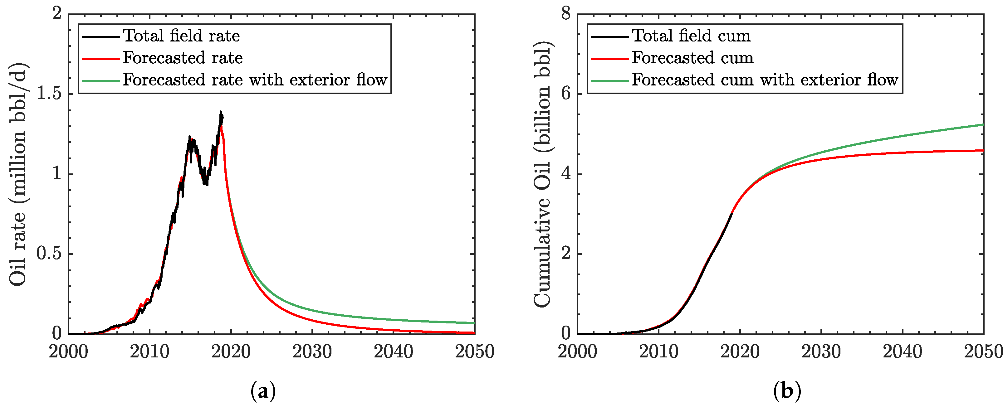
We have replaced actual field production rate from all existing wells in each region with this region’s well prototype multiplied by the historic numbers of completed wells, and we time-shifted the products. The superposed prototypes match the historical field rate. Figure 7 shows the sum of the well prototypes with and without exterior flows (green and red lines) versus the total field historical oil rate and cumulative oil (black lines). The results are rather satisfactory. Our GEV prototypes are robust. They capture all peaks of total historical oil rate and flawlessly match the cumulative production. As stated before, the red line forecast is pessimistic. It assumes that there will be no production contribution from the reservoir exterior to the SRVs of individual wells. This pessimistic case may hold if a shale play, here Bakken, is already overdrilled. For the Bakken shale, we can infer that the 14,678 existing wells will ultimately produce 4.5–5.3 billion of oil by 2050. This is a ‘base’ or ‘do nothing’ case with no future drilling in the Bakken shale.
2.5. Infill Potentials
We have calculated the number of wells that can be drilled in the future in every one-square-mile pixel of the grid that covers the entire Bakken play. In order to calculate infill potentials, one should first determine well density. However, the publicly available data rarely provide information about the bottomhole locations of the wells. Instead, only surface locations are reported as latitude-longitude coordinates. Therefore, we have developed an algorithm that allows us to predict the bottomhole well density from surface well locations. See Figure 8 and the Materials and Methods section for more details. As mentioned before in Section 2.1, the Bakken shale has two reservoirs, the Middle Bakken and Three Forks and two significantly different reservoir qualities, the core and noncore areas. Thus the infill potentials should be calculated for these four parts of the Bakken. Supporting Online Materials-2 shows the gridding, well locations, wellhead densities, well densities and infill potentials for the four Bakken parts. Table 3 lists the numbers of wells that can potentially be drilled in the future. We note in passing that infilling the less productive noncore areas to the same well density as the core areas is likely too optimistic.
2.6. Future Drilling Scenarios and Infill Forecasts
We have created several future drilling scenarios based on infill potentials listed in Table 3. We assume that the rig count in the Bakken will not significantly change from the current value and 120 wells will be drilled each month between now and 2041 (Figure 9a). By looking at the current trend, many operators have narrowed their drilling choices to only the core areas to avoid spending money on the less productive wells with high watercuts typical of the noncore areas [22]. Thus, it is reasonable to create a drilling schedule that exhausts all potential wells in the core areas first, before moving out to the less productive noncore areas. Figure 9b shows this scenario predicting that the Bakken core area will be completely drilled out by 2022. Later, the drilling in noncore areas can last up to 2041, according to our calculation. See Supporting Online Materials-2 for the more detailed schedules.
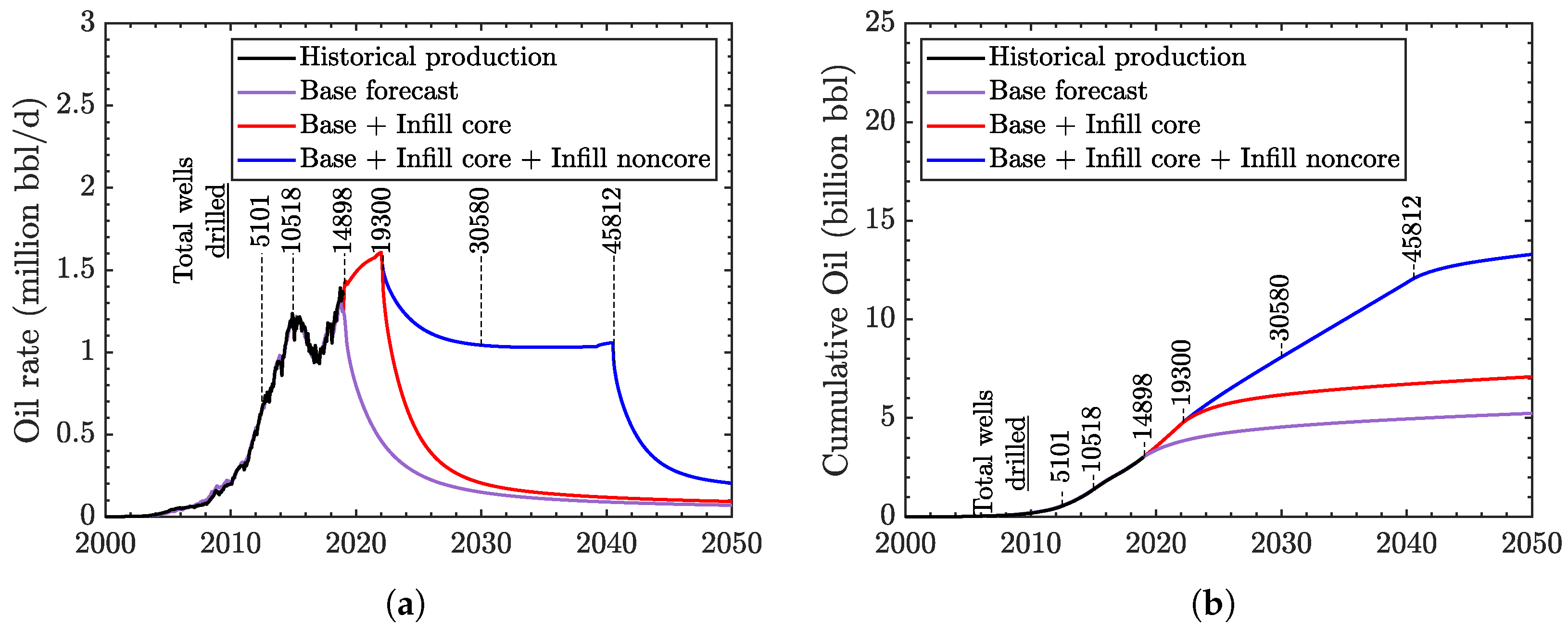
Next, we assign each new well scheduled to be drilled in the future to its corresponding region and class prototype. The results are shown in Figure 10. The black solid lines are the historical total field oil rate and cumulative oil. The purple lines denote the ‘base’ forecast from all 14,678 existing wells displayed in Section 2.4. The red lines show the result of adding 4402 new wells in the core area. Because all wells in the core area are high-grade wells, the total oil production rate climbs up its highest production peak at 1.6 million bbl/d in the year 2022. After 2022, there is no further drilling in the core area and the production rate declines by a factor of two within one year. Ultimately, the total of 19,080 wells (existing + new core) will produce 7 billion bbl of oil by the year 2050. The blue lines show the most optimistic case with not only the core areas but also the noncore areas will be drilled out by the operators. The drilling of less productive wells in the noncore areas will maintain the plateau oil rate of 1 million bbl/d up to the year 2041. However, this plateau will require the drilling of additional 26,500 wells (almost twice the current number of wells) which will have high water cuts. Ultimately, the total of 45,580 wells (existing + core + noncore) will produce 13 billion bbl of oil by 2050.
3. Discussion
We have presented an alternative to the current industry-standard empirical forecasts of oil production from hydrofractured horizontal wells in shales. With our hybrid modeling approach, we have matched current oil production in the Bakken rather accurately. We have also delivered an optimal prediction of possible futures of the Bakken shale play for up to three decades.
Our Bakken oil forecasting method extends the previous work on predicting fieldwide gas production in the Barnett shale [21] and merges it with our new scaling of oil production in the Bakken [22]. Our field data-driven statistical well prototypes are conditioned by well attrition, hydrofracture deterioration, pressure interference, well interference, progress in technology, and so forth. With no physical scaling, these prototypes follow the exact physics of linear transient oil flow with pressure interference. Therefore these statistical well prototypes serve as templates to calibrate the parameters of our physical scaling model ( and [23,24] and obtain a smooth time-extrapolation of oil production that is mechanistic and not merely an empirical decline curve. At late times, we add to our extended prototypes some radial inflow from the outside of well SRVs [26].
The extended well prototypes in Figure 6 can be used to compare ultimate recovery in each of the static regions we have identified in the Bakken. The lower bounds are the extended prototypes without exterior flow (red lines). In most cases, wells completed in the upper Three Forks reservoir are somewhat less productive than those in the Middle Bakken reservoir. The reasons for this difference are: (1) higher water saturation and water cut in Three Forks, (2) faster decline rate (lower ) and (3) lower initial oil in place (lower ) [22]. This difference is consistent with the stratigraphic column of the Bakken total petroleum system, where Middle Bakken is sandwiched between two world-class source rocks with 10% TOC, the Upper Bakken Shale and the Lower Bakken Shale. On the other hand, the Three Forks formation is below the Lower Bakken Shale member and is exposed to water-bearing formations beneath [3,28,29,30]. For the same reasons, the core and effective drilling areas in the Three Forks are smaller than those in the Middle Bakken.
In both reservoirs, production from the core areas is superior to that from the noncore areas. The core area located in the center of Williston Basin has been known as the most oil-prolific location in the Bakken region in North Dakota [3,28,29,30]. Since the 1950s, oil has been produced there in the thickest, naturally fractured Middle Bakken formation in the Nesson anticline. One inexpensive vertical well drilled in the core area in the 1950s has had ultimate recovery of 200 kbbl, the same as a $10 million hydrofractured horizontal well drilled in the Middle Bakken noncore area nowadays. The noncore areas are less productive because the three Bakken formations: Upper, Middle and Lower Bakken are pinching out upward (are thinner and less mature) near the edges of the Williston basin. Consequently, the noncore areas are producing more water than oil, with watercut exceeding 50% on average.
The newly completed wells have much higher initial oil rates than the older ones, because they have: (1) longer lateral lengths, (2) bigger hydraulic fractures and (3) more fracture stages [22,31,32,33,34]. However, the newly completed wells decline faster and have essentially the same ultimate recovery as the older wells. The reasons for this behavior have been described elsewhere [35]. Interestingly, in most cases, older wells completed in 2000–2012 have higher ultimate recovery than newer ones, even though their initial production rates are lower. These older wells might have been drilled in the best locations ever in the Bakken region. In addition, shorter lateral lengths and fewer fracture stages may help in maintaining a stable pressure drawdown and prevent reservoir degassing that is unfavorable for future production. For comparison, the average lateral length in 2005 was 5000 ft while the average lateral length in 2019 doubled to 10,000 ft. Historically, the number of hydrofracture stages in the Bakken has increased over time from 8 stages in 2007 [36] to 18 stages in 2009 [31], 35 stages in 2016 [32] and to as many as 60 stages in 2019 [33].
According to our records, more than 90% of the wells completed after 2017 are located in the core areas only. Operators have learned to drill only the best parts of the Williston Basin and avoid the less mature noncore areas. However, after calculating the infill potentials of all areas, we predict that by 2021 there will be no well locations left for future drilling in the core areas. Assuming a constant current drilling rate of 120 wells per month, the total field oil rate in the Bakken will reach record level of about 1.6 million bbl/d in 2021. Without further drilling, production will decline by one-half within a year. Later, operators will be forced to drill in the less productive, high watercut noncore areas along the edges of the Williston Basin. Our findings suggest that policy-makers should not assume that the shale oil boom in the Bakken will last for several decades longer. We recommend that operators not focus only on increasing the initial oil rate. Maintenance of reservoir pressure above the bubble point by preventing over-drilling is key to increasing ultimate oil recovery.
4. Materials and Methods
We mined public well data in the Bakken region from DrillingInfo database, the Montana Department of Natural Resources and Conservation–Board of Oil and Gas Conservation website and the North Dakota Department of Mineral Resources–Oil and Gas Division website. From DrillingInfo, we selected only 14,678 horizontal oil wells that were completed in the Middle Bakken and Three Forks formations after January 2000. We designed an integrated MATLAB software package to perform data cleanup, consolidation and unit conversions. The clean production data for each well consist of a vector of elapsed times on production, vector of oil and water production rates and records of wellhead location (latitude and longitude), lateral length, completion date, reservoir description and maximum oil rate. The average reservoir and well lateral properties are listed in Appendix C. Our approach can be divided into six main steps:
- Define play regions in which oil production is statistically uniform. In each region, follow the steps below:
- (a)
- Divide all wells in a play into well groups, where n is the number of reservoirs. In the Bakken play, for example, there are two main reservoirs. Thus, at this step, we identify two groups of wells,
and in the Bakken shale.Well Sample Reservoir Sample Size 1 Middle Bakken 9860 2 Three Forks 4818 - (b)
- Further subdivide each of these well groups into , , areas with different reservoir qualities. For example, in the Bakken play, the center of the basin has the thickest oil-prolific layer and hence the highest oil production [3,22,28,29,30]. Thus, we have delineated an area at the center of the basin (with maximum oil rate >750 bopd) as core area and the rest as area, see Figure 2 for more details. At this step, we have four well groups that fall into four distinct, static play regions,
In Bakken, and , that is, there are two reservoir qualities (core and noncore) for each of the reservoirs (Middle Bakken and Three Forks).Reservoir Region Sample Size 1 Middle Bakken core 5732 2 Middle Bakken noncore 4128 3 Three Forks core 2672 4 Three Forks noncore 2146 - (c)
- Subdivide wells in each of the four regions (two reservoirs × two reservoir qualities each) by time interval classes that encompass significant changes in well completion technology. In the Bakken play, for instance, the newly completed wells have longer lateral lengths, bigger hydraulic fractures and more fracture stages [22,31,32,33,34]. Thus, we classify the wells in each of the four regions by three completion date intervals: [2000–2012], [2013–2016] and [2017–2019]. In the end, we have divided all 14,678 horizontal wells in the Bakken into 12 well groups (4 regions × 3 completion date classes) listed in Table 1. In Bakken, each of the 4 play regions has 3 completion classes, finally yielding 12 static well samples.
- For each well sample, obtain a well prototype by fitting a Generalized Extreme Value (GEV) distribution to all qualifying sample wells as follows:
- (a)
- From a given static well sample-k (a region further subdivided by completion dates), consider a dynamic cohort that contains all wells that have at least years on production ( and ). For example: (i) There are 2550 wells in Middle Bakken noncore [2000–2012] group. However, there are only 2540 wells with at least one year on production (the other 10 wells have production records with less than 12 months). Thus, we retain these 2540 wells as cohort-1 of this particular group, see Figure 4. (ii) There are 428 wells in Three Forks core [2000–2012] group. But, only 197 wells have production records of at least seven years. As such, these 197 wells are qualified as cohort-7 of this particular well group, see Figure 5. For detailed GEV fits for all dynamic well cohorts and static well groups in the Bakken play, see Supporting Online Materials-1. For Bakken, .
- (b)
- Define a set that takes values of oil production rate (kbbl/year) from all wells with at least years on production in sample k.
- (c)
- For every , fit a Generalized Extreme Value (GEV) distribution using Equation (A1) and obtain the location parameter, , scale parameter, and shape parameter, . (All of these parameters are further subscripted by but we will skip this complication in the notation.)
- (d)
- Calculate as the GEV mean of for each year-, , using Equation (A3).
- (e)
- For each well sample k, obtain the well prototype. We can use the same procedure to obtain other statistic parameters for each well cohort. The and values can be calculated as the ninetieth and tenth percentiles of , respectively. The median and mode can be calculated using Equations (A5) and (A6). by connecting GEV mean values of all years
- Extend (we will subsequently skip the implied subscript k) well prototypes by fitting to them physical scaling curves as follows:
- (a)
- For a each well sample k, calculate the observed cumulative mass produced, (ktons) from Equation (A13). Fix in kbbl/year and year.
- (b)
- Adjust in Equation (A22) or Equation (A7) (with or without exterior flow) and in Equation (A11), so that the physical scaling curve matches the observed . Use and a values from the average Bakken reservoir properties listed in Table A1 and Table A2. The matching values of and for two both scaling curves and for all well samples are detailed in Table 2.
- (c)
- Get the extended cumulative mass produced, (ktons) by multiplying the fitted and from the master curve where t is now calculated each month The benefit of matching with a physics-based scaling curve is that we can interpolate and extrapolate production data precisely. Thus, we can change time intervals from years to months and forecast production decades into the future. We recommend to use monthly intervals for precise forecasts that is, years.
- (d)
- Obtain the extended well prototypes for well sample k by differencing converted to volume
- Obtain base forecast of total field oil production for existing wells as follows:
- (a)
- Create a calendar date series with monthly intervals for example, (1/1/2000, 2/1/2000, ⋯, 12/1/2050) and assign as the length of this series.
- (b)
- Create an empty vector with the length of : ().
- (c)
- For each well, find index in the calendar date series that brackets well completion date.
- (d)
- For each well, add to vector its corresponding right-shifted by .
- (e)
- Calculate total field oil rate, and total field cumulative oil, for existing wells as follows:
- Calculate infill potential as follows:
- (a)
- Create a one-square-mile fishnet inside the boundary of each area defined in step I(b).
- (b)
- Search all existing wells located inside the boundary.
- (c)
- Calculate wellhead density by counting the number of wells on each of the one-square-mile squares.
- (d)
- Calculate approximate well density following algorithm below.
- For each well, calculate the number of squares, n, intercepted by the lateral For example, a 5000 ft lateral occupies one square, a 9000 ft lateral occupies two squares and a 14,000 ft lateral occupies three squares because one mile is 5280 ft.
- Search for the least-occupied n squares in all possible directions.
- Increase the value of well density by 1 well/mi for every least dense n square found.
- Repeat points i–iii until all wells in the area of interest are exhausted.
- (e)
- Calculate infill potential by subtracting the calculated well density from the maximum allowable number of wells that still avoid frac hits. For example, in the Bakken play, the tip-to-tip hydraulic fracture length is roughly 1200 ft. 5280 ft/1200 ft ≈ 4. Therefore, the maximum allowable number of wells to avoid frac hits is 4 wells per square mile. Suppose that at some location, the well density already is 3 wells per square mile. Then, the infill potential is well per square mile.
- Obtain an infill forecast of total field oil production after adding future wells.
- (a)
- Create monthly drilling schedules for every infill potential and assume a constant drilling rate based on current rig availability, see Figure 9b and SOM-2.
- (b)
- Use the same calendar date series as in step IV(a) with as the length of date series.
- (c)
- Create an empty vector with the length of ().
- (d)
- For every drilling schedule, find index in the calendar date series that brackets infill schedule date. Let be the number of wells to be drilled on that date.
- (e)
- For every drilling schedule, add to vector its corresponding after right-shifting it by and multiplying by .
- (f)
5. Conclusions
- We have provided a transparent hybrid method of forecasting oil production at shale basin scale.
- Our statistical approach generates the non-parametric well prototype templates that are used to calibrate our physics-based flow scaling with late-time radial inflow.
- In particular, our average well prototypes follow the physics of linear transient flow and are used to calibrate the physics-based scaling extensions to 30 years on production.
- A combination of GEV statistics with physical scaling matches historical production data almost perfectly and gives a smooth, physics-based estimate of future production.
- Regulators may want to consider our approach as a prerequisite to booking reserves in oil shales.
- Newly completed wells have almost the same ultimate recovery as the older ones, despite their much higher initial oil rates.
- Ultimately, we predict that the 14,678 existing wells in the Bakken will produce 5 billion bbl of oil by 2050 (∼340 kbbl/well).
- After drilling additional 4400 new wells at the rate of 120 wells/month, the core area of the Bakken will be drilled out by 2021 and ultimate recovery will be 7 billion barrels of oil.
- With 26,500 more wells to be drilled in the noncore area until 2041, ultimate recovery in the Bakken might be 13 billion barrels of oil but drilling of such scale is unlikely to happen.
- Policy-makers should not of assume that oil boom in the Bakken shale will last decades longer.
Supplementary Materials
The following are available online at https://www.mdpi.com/1996-1073/12/19/3641/s1. There are two files. The first one shows full details of infill potential maps for every sub-region in the Bakken shale and a table listing drilling schedule program until year 2050. The second file shows 225 unique plots showing all the GEV distributions used to match all well cohorts in the Bakken shale.
Author Contributions
Conceptualization, T.P. and W.S.; methodology, T.P. and W.S.; software, W.S. and T.P.; validation, T.P. and W.S.; formal analysis, W.S. and W.K.; investigation, W.K. and W.S.; resources, T.P.; data curation, W.K.; writing–original draft preparation, W.S.; rewriting manuscript–review and editing, T.P. and W.S.; visualization, W.S.; supervision, T.P. and W.K.; project administration, T.P.; funding acquisition, T.P.
Funding
Wardana Saputra (PhD student) was supported by baseline research funding from KAUST to Tad Patzek. Wissem Kirati (Research Engineer) was supported by the Division of Computer, Electrical and Mathematical Science at KAUST.
Acknowledgments
The authors thank the Ali I. Al-Naimi Petroleum Engineering Research Center (ANPERC) at KAUST for supporting this research. We thank the reviewers for their thorough, informative and timely reviews.
Conflicts of Interest
The authors declare no conflict of interest.
Abbreviations
The following abbreviations are used in this manuscript:
| CDF | Cumulative Distribution Function |
| EUR | Estimated Ultimate Recovery |
| GEV | Generalized Extreme Value |
| Probability Density Function | |
| SRV | Stimulated Reservoir Volume |
Appendix A. The Generalized Extreme Value (GEV) Distributions
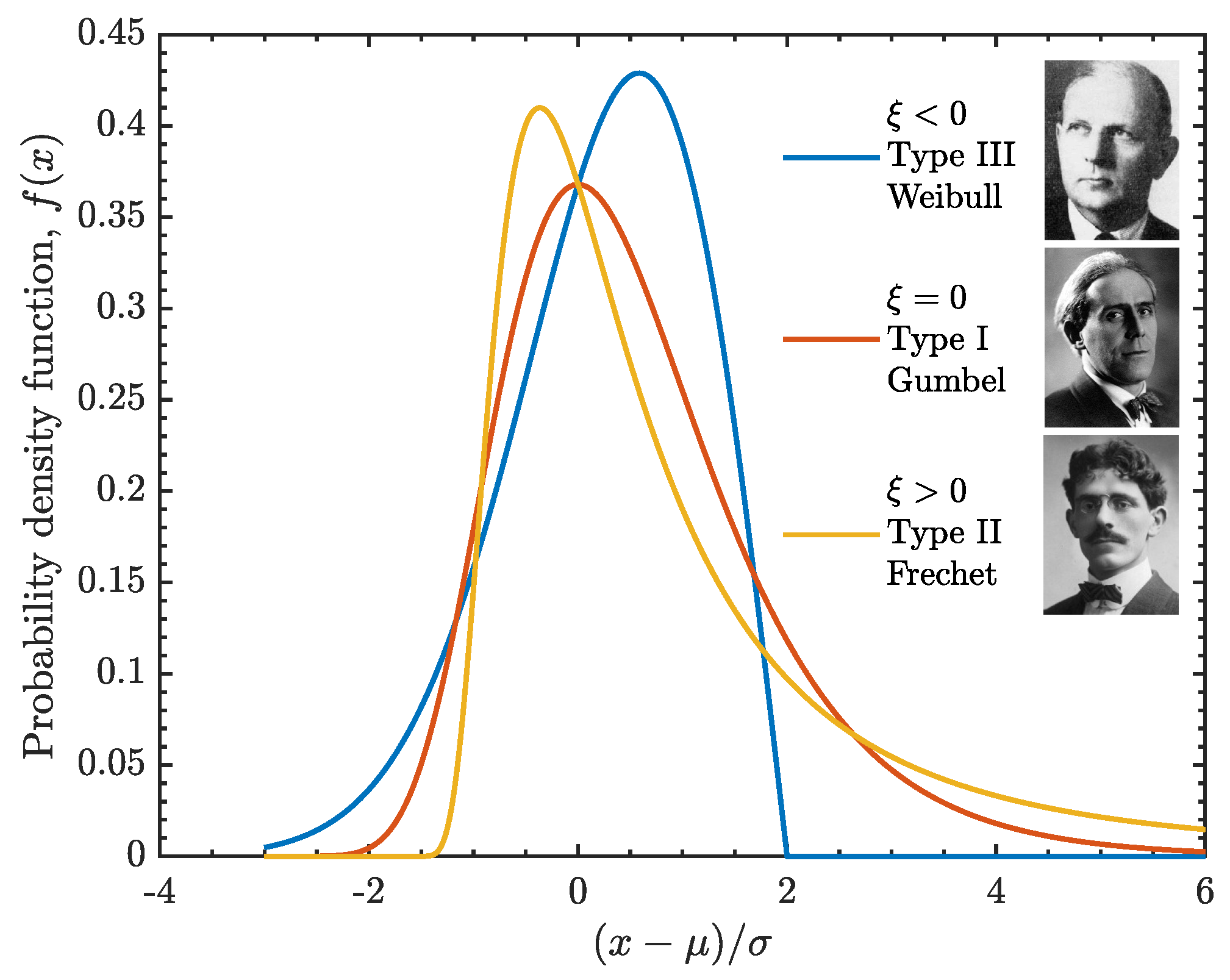
The Generalized Extreme Value (GEV) distribution [41] combines three “Extreme Value" distributions, Weibull [42], Gumbel [43] and Frechet [44] into a single functional form. The data decide which of the three distributions is appropriate. In our case, Fréchet distribution almost always wins.
The probability density function (PDF) of GEV distribution contains three parameters: location, ; scale, ; and shape,
If is zero, Gumbel distribution results, followed by Weibull distribution, if is negative and by Fréchet distribution if is positive (Figure A1).
Integrating the GEV PDF, one obtains the cumulative distribution function (CDF)
The expected value (mean) of GEV distribution is defined as
and the variance is
where and is Euler’s constant. Notice that for , the expected value becomes infinite and for the variance goes to infinity.
Figure A1.
Examples of three GEV distributions with the location parameter, , the scale parameter, . and three values of the shape parameter i.e., (Weibull), (Gumbel) and (Fréchet).
Figure A1.
Examples of three GEV distributions with the location parameter, , the scale parameter, . and three values of the shape parameter i.e., (Weibull), (Gumbel) and (Fréchet).

The median of GEV distribution is defined as
and the mode is
Appendix B. Physical Scaling Approach to Forecasting Oil Production in Hydrofractured Shales
The physical scaling approach used in this paper was first derived by Patzek et al. to predict gas production from thousands of hydrofractured horizontal gas wells in the Barnett shale [23,24]. Later, Patzek et al. derived the scaling curve solution for oil production in the Eagle Ford shale [25]. Eftekhari et al. extended the model to include gas inflow from outside of SRVs for the Barnett shale wells [26].
Appendix B.1. Physical Scaling without Exterior Flow
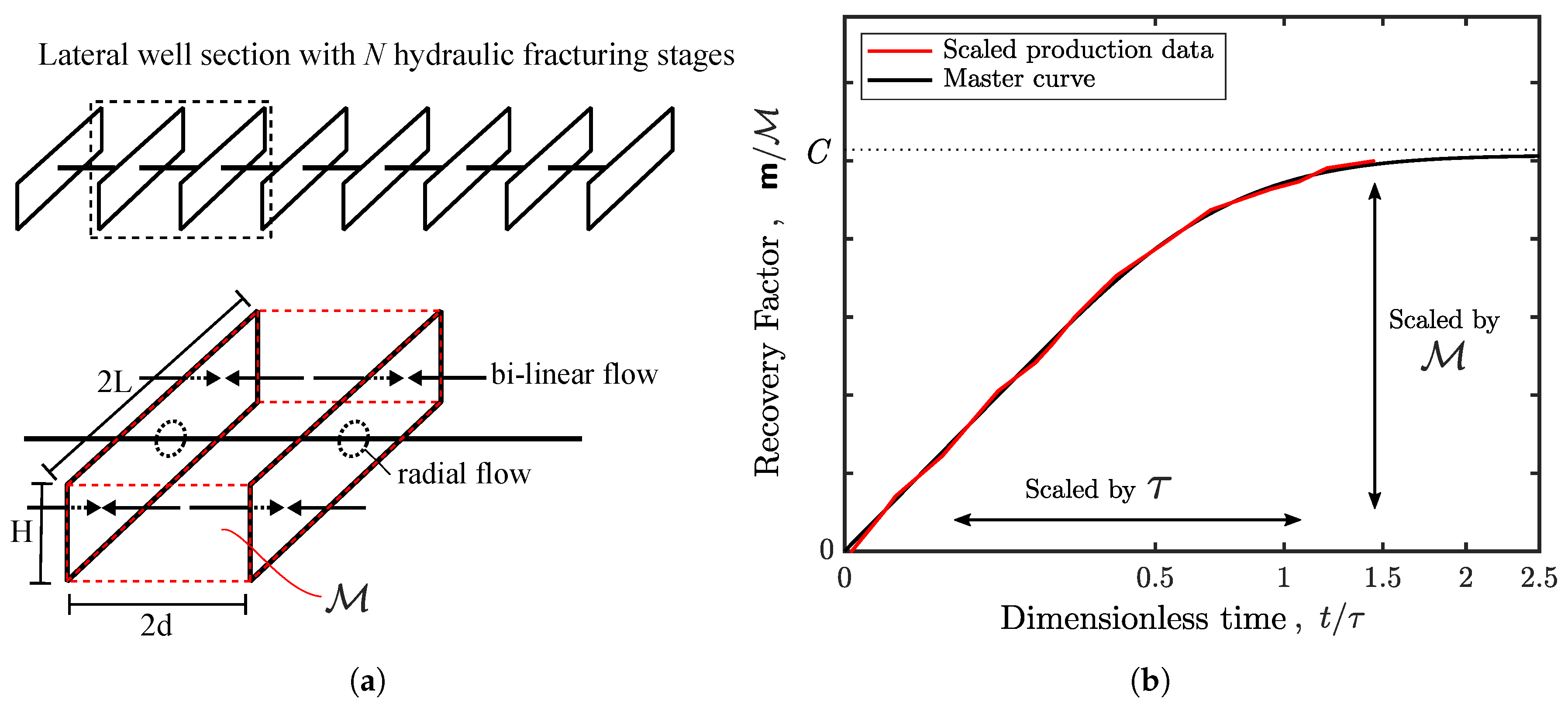
Patzek et al. [25] derived the solution of oil production inside SRV based on a simple model illustrated in Figure A2a. This model assumes bi-linear flow towards hydraulic fracture planes inside SRV with the volume . Briefly, by solving a one-dimensional nonlinear pressure diffusion equation analytically, we obtain a master curve equation for the interior oil production problem
where is the dimensionless time defined as the ratio between elapsed time on production, t and the characteristic time of pressure diffusion, .
Here is determined by the onset of pressure interference between two hydrofractures apart
and is the constant hydraulic diffusivity at initial reservoir conditions
Figure A2.
(a) Schematic of bi-linear flow towards hydraulic fractures in a shale well inside the SRV with volume H × 2d × 2L (interior problem). The early radial flow is neglected because the hydrofracture permeability is much higher than that of the matrix. Reproduced from Patzek et al. [25] (b) Illustration of physical scaling approach of the interior oil production problem. Reproduced from Saputra et al. [27].

The fractional oil recovery factor, RF, is the ratio between the cumulative oil mass production, and the stimulated mass contained in the SRV,
where
and
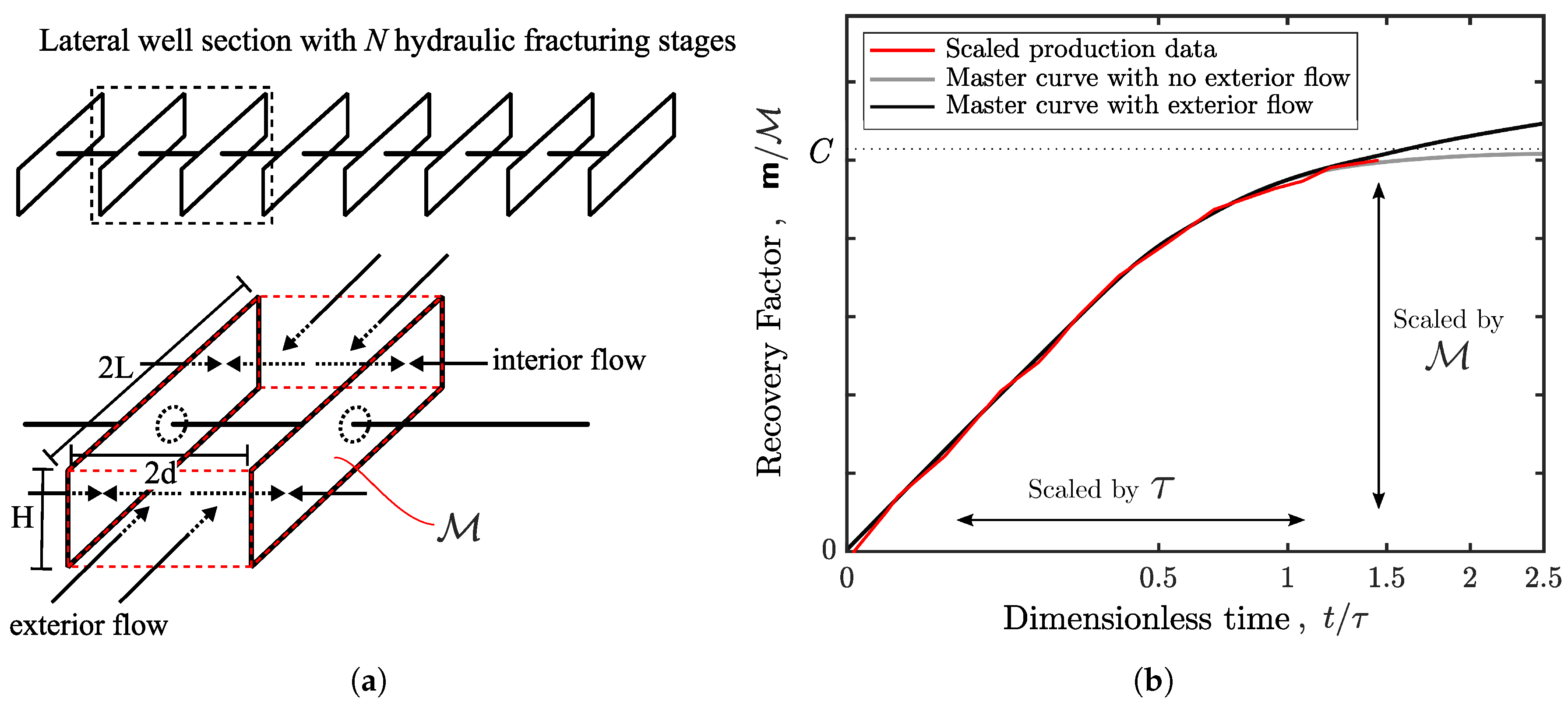
Appendix B.2. Physical Scaling with Exterior Flow
Eftekhari et al. [26] solved numerically the exterior gas production problem in the Barnett shale. We later extended the same concept to oil shales and proposed an analytical solution of this problem. Figure A3a illustrates interior flow towards the hydraulic fractures inside SRV and exterior flow from the outer reservoir towards SRV. We write a new master curve equation for both interior and exterior flow as follows
where is the master curve equation for interior oil production problem (Equation (A7)). Eftekhari et al. [26] defined the recovery factor of the exterior problem as a function of the new scaled time, where is the cumulative exterior production and is the stimulated mass inside SRV defined in Equation (A12)
Here is the characteristic time scale for exterior production, defined as the time it takes low pressure to diffuse from the wellbore over a distance equal to fracture half-length L
The new scaled time for exterior production, can be written as a function of the interior scaled time, in Equation (A8):
Because oil flow from the exterior reservoir is another one-dimensional pressure diffusion problem, one can assume the square root of time solution [26] with a constant slope
Because both the interior and exterior reservoir likely contain similar shale matrix with similar reservoir properties, the constant can be assumed to be the slope of the interior master curve versus square-root of time (Equation (A7) and Figure A2b), which is constant at early times, say, .
can be written as a function of the scaled time for the interior production by substituting Equations (A17) and (A18):
where a is defined as
Recalling Equation (A14), we obtain a new master curve equation that embodies interior and exterior oil flow as follows
Figure A3.
(a) Illustration of interior flow towards the hydraulic fractures of a shale well inside SRV and exterior flow from the reservoir beyond SRV. Adapted from Patzek et al. [25] and Eftekhari et al. [26] (b) Illustration of physical scaling approach of the interior and exterior oil production problem. Adapted from Saputra et al. [27].

The physical scaling approach for this problem is as follows. By adjusting and , minimize the square of the difference of minus the cumulative mass produced with Equation (A13). A least square fit procedure was used. Figure A3b shows the scaled cumulative mass as the red line and the new master curve as the black line that deviates from the interior master curve in Equation (A7) (shown as the gray line) at late times on production.
Appendix C. Reservoir Properties of the Bakken Shale

Table A1.
Reservoir properties used in scaling oil production in the Middle Bakken and Three Forks (part-1).
Table A1.
Reservoir properties used in scaling oil production in the Middle Bakken and Three Forks (part-1).
| Parameter | Middle Bakken | Three Forks | Data Source | ||
|---|---|---|---|---|---|
| SI Units | Field Units | SI Units | Field Units | ||
| Initial pressure, | 36.8 Mpa | 5340 psia | 37.1 Mpa | 5380 psia | [22] |
| Fracture pressure, | 3.4 Mpa | 500 psia | 3.4 Mpa | 500 psia | [22] |
| Connate water saturation, | 0.57 | 0.57 | 0.65 | 0.65 | [22] |
| Initial oil saturation, | 0.43 | 0.43 | 0.35 | 0.35 | [22] |
| Rock porosity, | 0.046 | 0.046 | 0.058 | 0.058 | [22] |
| Rock permeability, k | 4.4 × m | 0.045 md | 4.6 × m | 0.047 md | [22] |
| Rock compressibility, | 4.3 × Pa | 3.0 × psi | 4.3 × Pa | 3.0 × psi | [45] |
| Water compressibility, | 4.3 × Pa | 3.0 × psi | 4.3 × Pa | 3.0 × psi | [45] |
| Oil compressibility, | 1.4 × Pa | 1.0 × psi | 1.4 × Pa | 1.0 × psi | [45] |
| Total compressibility, | 6.3 × Pa | 9.0 × psi | 5.9 × Pa | 8.5 × psi | |
| Oil viscosity, | 3.9 × Pa s | 0.392 cp | 2.8 × Pa s | 0.276 cp | [46] |
| API gravity | 42.2API | 42.2API | 38.7API | 38.7API | [46] |
| 0.1014 | 0.1014 | 0.1178 | 0.1178 | ||
Table A2.
Reservoir properties used in scaling oil production in the Middle Bakken and Three Forks (part-2).
References
- Arps, J.J. Analysis of decline curves. Trans. AIME 1945, 160, 228–247. [Google Scholar] [CrossRef]
- Zuo, L.; Yu, W.; Wu, K. A fractional decline curve analysis model for shale gas reservoirs. Int. J. Coal Geol. 2016, 163, 140–148. [Google Scholar] [CrossRef]
- Gaswirth, S.B.; Marra, K.R.; Cook, T.A.; Charpentier, R.R.; Gautier, D.L.; Higley, D.K.; Klett, T.R.; Lewan, M.D.; Lillis, P.G.; Schenk, C.J. Assessment of undiscovered oil resources in the Bakken and Three Forks formations, Williston Basin Province, Montana, North Dakota, and South Dakota, 2013. US Geol. Surv. Fact Sheet 2013, 3013, 1–4. [Google Scholar]
- Cook, T.A. Procedure for Calculating Estimated Ultimate Recoveries of Bakken and Three Forks Formations Horizontal Wells in the Williston Basin; US Geol. Surv. Open-File Report; U.S. Geological Survey: Reston, VA, USA, 2013; pp. 1–14.
- EIA. Assumptions to the Annual Energy Outlook 2019: Oil and Gas Supply Module. US Energy Inf. Adm. Annu. Energy Outlook 2019, 7, 4–7. [Google Scholar]
- Hughes, J. A reality check on the shale revolution. Nature 2013, 494, 307–308. [Google Scholar] [CrossRef] [PubMed]
- Hughes, J. 2016 Tight Oil Reality Check; Post Carbon Institude: Santa Rosa, CA, USA, 2016. [Google Scholar]
- Hughes, J. Shale Reality Check; Post Carbon Institude: Santa Rosa, CA, USA, 2018. [Google Scholar]
- Hughes, J. How Long Will the Shale Revolution Last? Technology Versus Geology and the Lifecycle of Shale Plays; Post Carbon Institude: Santa Rosa, CA, USA, 2019. [Google Scholar]
- Ilk, D.; Anderson, D.M.; Stotts, G.W.; Mattar, L.; Blasingame, T. Production Data Analysis–Challenges, Pitfalls, Diagnostics. SPE Reserv. Eval. Eng. 2010, 13, 538–552. [Google Scholar] [CrossRef]
- Valko, P.; Lee, W. A Better Way To Forecast Production From Unconventional Gas Wells. In Proceedings of the SPE Annual Technical Conference and Exhibition, Florence, Italy, 19–22 September 2010. [Google Scholar]
- Clark, A.J.; Lake, L.W.; Patzek, T.W. Production forecasting with logistic growth models. In Proceedings of the SPE Annual Technical Conference and Exhibition, Denver, CO, USA, 30 October–2 November 2011. [Google Scholar]
- Zhang, H.; Rietz, D.; Cagle, A.; Cocco, M.; Lee, J. Extended exponential decline curve analysis. J. Nat. Gas Sci. Eng. 2016, 36, 402–413. [Google Scholar] [CrossRef]
- Du, D.; Zhao, Y.; Guo, Q.; Guan, X.; Hu, P.; Fan, D. Extended Hyperbolic Decline Curve Analysis in Shale Gas Reservoirs. In Proceedings of the International Field Exploration and Development, Chengdu, China, 21–22 September 2017; pp. 1491–1504. [Google Scholar]
- Gong, X.; Gonzalez, R.; McVay, D.A.; Hart, J.D. Bayesian probabilistic decline-curve analysis reliably quantifies uncertainty in shale-well-production forecasts. SPE J. 2014, 19, 1–47. [Google Scholar] [CrossRef]
- Yu, W.; Tan, X.; Zuo, L.; Liang, J.; Liang, L. A new probabilistic approach for uncertainty quantification in well performance of shale gas reservoirs. SPE J. 2016, 21, 2038–2048. [Google Scholar] [CrossRef]
- Paryani, M.; Awoleke, O.O.; Ahmadi, M.; Hanks, C.; Barry, R. Approximate Bayesian Computation for Probabilistic Decline-Curve Analysis in Unconventional Reservoirs. SPE Reserv. Eval. Eng. 2017, 20, 478–485. [Google Scholar] [CrossRef] [Green Version]
- Fulford, D.S.; Bowie, B.; Berry, M.E.; Bowen, B.; Turk, D.W. Machine learning as a reliable technology for evaluating time/rate performance of unconventional wells. SPE Econ. Manag. 2016, 8, 23–39. [Google Scholar] [CrossRef]
- de Holanda, R.W.; Gildin, E.; Valkó, P.P. Mapping the Barnett Shale Gas with Probabilistic Physics-Based Decline Curve Models and the Development of a Localized Prior Distribution. In Proceedings of the Unconventional Resources Technology Conference, Houston, TX, USA, 23–25 July 2018; pp. 217–232. [Google Scholar]
- Holanda, R.W.d.; Gildin, E.; Valko, P.P. Combining physics, statistics, and heuristics in the decline-curve analysis of large data sets in unconventional reservoirs. SPE Reserv. Eval. Eng. 2018, 21, 683–702. [Google Scholar] [CrossRef]
- Patzek, T.W.; Saputra, W.; Kirati, W.; Marder, M. Generalized Extreme Value Statistics, Physical Scaling and Forecasts of Gas Production in the Barnett Shale. Energy Fuels 2019. in review. Available online: https://doi.org/10.26434/chemrxiv.8326898.v1 (accessed on 27 June 2019).
- Saputra, W.; Kirati, W.; Patzek, T.W. Prediction of ultimate recovery in the existing Bakken Shale wells using a physical scaling approach. J. Petr. Sci. Eng. 2019. in review. [Google Scholar]
- Patzek, T.W.; Male, F.; Marder, M. Gas production in the Barnett Shale obeys a simple scaling theory. Proc. Natl. Acad. Sci. USA 2013, 110, 19731–19736. [Google Scholar] [CrossRef] [Green Version]
- Patzek, T.; Male, F.; Marder, M. A simple model of gas production from hydrofractured horizontal wells in shales. AAPG Bull. 2014, 98, 2507–2529. [Google Scholar] [CrossRef]
- Patzek, T.; Saputra, W.; Kirati, W. A Simple Physics-Based Model Predicts Oil Production from Thousands of Horizontal Wells in Shales. In Proceedings of the SPE Annual Technical Conference and Exhibition, San Antonio, TX, USA, 9–11 October 2017. [Google Scholar]
- Eftekhari, B.; Marder, M.; Patzek, T.W. Field data provide estimates of effective permeability, fracture spacing, well drainage area and incremental production in gas shales. J. Nat. Gas Sci. Eng. 2018, 56, 141–151. [Google Scholar] [CrossRef]
- Saputra, W.; Albinali, A.A. Validation of the Generalized Scaling Curve Method for EUR Prediction in Fractured Shale Oil Wells. In Proceedings of the SPE Kingdom of Saudi Arabia Annual Technical Symposium and Exhibition, Dammam, Saudi Arabia, 3–26 April 2018. [Google Scholar]
- Sonnenberg, S.A.; Pramudito, A. Petroleum geology of the giant Elm Coulee field, Williston Basin. AAPG Bull. 2009, 93, 1127–1153. [Google Scholar] [CrossRef]
- Mason, J. Oil production potential of the North Dakota Bakken. Oil Gas J. 2012, 110, 1–12. [Google Scholar]
- Meissner, F.F. Petroleum geology of the Bakken Formation Williston Basin, North Dakota and Montana. In 1991 Guidebook to Geology and Horizontal Drilling of the Bakken Formation; Montana Geological Society: Butte, MT, USA, 1991. [Google Scholar]
- Buffington, N.; Kellner, J.; King, J.G.; David, B.L.; Demarchos, A.S.; Shepard, L.R. New technology in the Bakken Play increases the number of stages in packer/sleeve completions. In Proceedings of the SPE Western Regional Meeting, Anaheim, CA, USA, 27–29 May 2010. [Google Scholar]
- Weddle, P.; Griffin, L.; Pearson, C.M. Mining the Bakken: Driving Cluster Efficiency Higher Using Particulate Diverters. In Proceedings of the SPE Hydraulic Fracturing Technology Conference and Exhibition, The Woodlands, TX, USA, 24–26 January 2017. [Google Scholar]
- Martin, E. United States Tight Oil Production 2018. Available online: www.allaboutshale.com/united-states-tight-oil-production-2018-emanuel-omar-martin (accessed on 25 March 2019).
- Weijermars, R.; van Harmelen, A. Shale Reservoir Drainage Visualized for a Wolfcamp Well (Midland Basin, West Texas, USA). Energies 2018, 11, 1665. [Google Scholar] [CrossRef]
- Haider, S.; Patzek, T.W. The key physical factors that yield a good horizontal hydrofractured gas well in mudrock. J. Nat. Gas Sci. Eng. 2019. Submitted. [Google Scholar] [CrossRef]
- Paneitz, J. Evolution of the Bakken Completions in Sanish Field, Williston Basin, North Dakota. In Proceedings of the SPE Applied Technology Workshop (ATW), Keystone, CO, USA, 6 August 2010. [Google Scholar]
- Chorin, A.J.; Kast, A.; Kupferman, R. Optimal prediction of underresolved dynamics. Proc. Natl. Acad. Sci. USA 1999, 95, 4094–4098. [Google Scholar] [CrossRef] [PubMed]
- Chorin, A.J.; Kast, A.; Kupferman, R. Unresolved computation and optimal prediction. Commun. Pure Appl. Math. 1999, 52, 1231–1254. [Google Scholar] [CrossRef]
- Chorin, A.J.; Kast, A.; Kupferman, R. On the prediction of large-scale dynamics using unresolved computations. Contemp. Math. 1999, 238, 53–75. [Google Scholar] [Green Version]
- Chorin, A.J.; Hald, O.; Kupferman, R. Optimal prediction and the Mori-Zwanzig representation of irreversible processes. Proc. Natl. Acad. Sci. USA 2000, 97, 2968–2973. [Google Scholar] [CrossRef] [PubMed]
- Gumbel, E.J. Statistics of Extremes; Columbia University Press: New York, NY, USA, 1958. [Google Scholar]
- Weibull, W. A statistical distribution function of wide applicability. J. Appl. Mech. 1951, 18, 293–297. [Google Scholar]
- Gumbel, E.J. Statistical theory of extreme values and some practical applications. NBS Appl. Math. Ser. 1954, 33, 1–60. [Google Scholar]
- Fréchet, M. Sur la loi de probabilité de l’écart maximum. Ann. Soc. Math. Polon. 1927, 6, 93–116. [Google Scholar]
- Tran, T.; Sinurat, P.D.; Wattenbarger, B.A. Production characteristics of the Bakken shale oil. In Proceedings of the SPE Annual Technical Conference and Exhibition, Denver, CO, USA, 30 October–2 November 2011. [Google Scholar]
- Kurtoglu, B. Integrated Reservoir Characterization and Modeling in Support of Enhanced Oil Recovery for Bakken; Colorado School of Mines: Golden, CO, USA, 2013. [Google Scholar]
Figure 1.
Division of the Bakken shale wells into 12 well samples.

Figure 2.
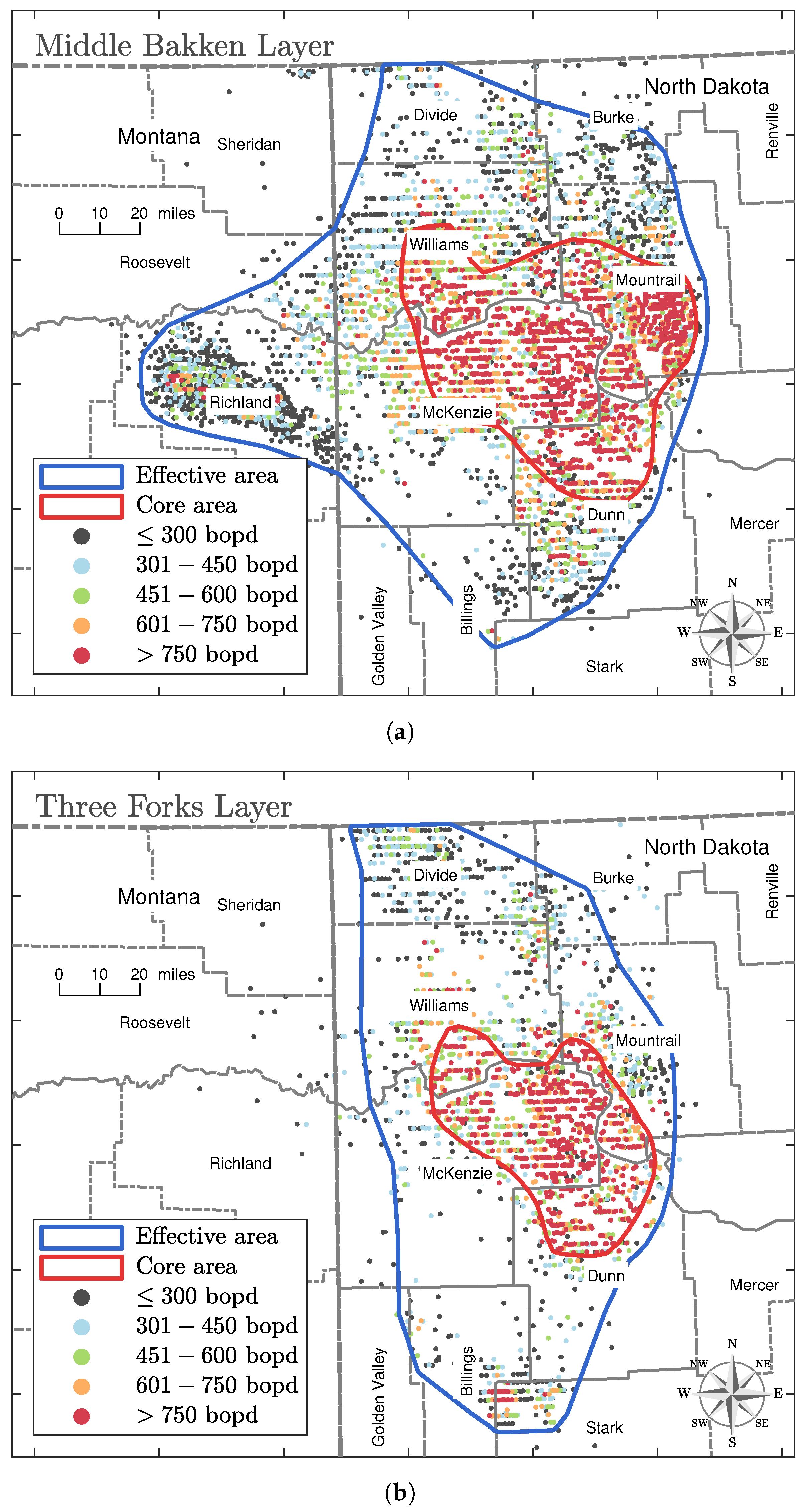
Maps of all 14,678 active horizontal wells completed in the Middle Bakken formation (a) and Three Forks formation (b) colored by maximum daily oil rate. The red lines define the core areas for each reservoir and delineate best producing wells with more than 750 barrels of oil per day. The blue lines define the effective areas for drilling neglecting a few poor producing wells outside. We define the noncore areas as the difference between the effective and core areas. In the Middle Bakken, there are currently 5732 and 4128 wells located in the core and noncore areas, respectively. The other 2672 and 2146 wells are located in the core and noncore areas of Three Forks, respectively.
Figure 2.
Maps of all 14,678 active horizontal wells completed in the Middle Bakken formation (a) and Three Forks formation (b) colored by maximum daily oil rate. The red lines define the core areas for each reservoir and delineate best producing wells with more than 750 barrels of oil per day. The blue lines define the effective areas for drilling neglecting a few poor producing wells outside. We define the noncore areas as the difference between the effective and core areas. In the Middle Bakken, there are currently 5732 and 4128 wells located in the core and noncore areas, respectively. The other 2672 and 2146 wells are located in the core and noncore areas of Three Forks, respectively.

Figure 3.
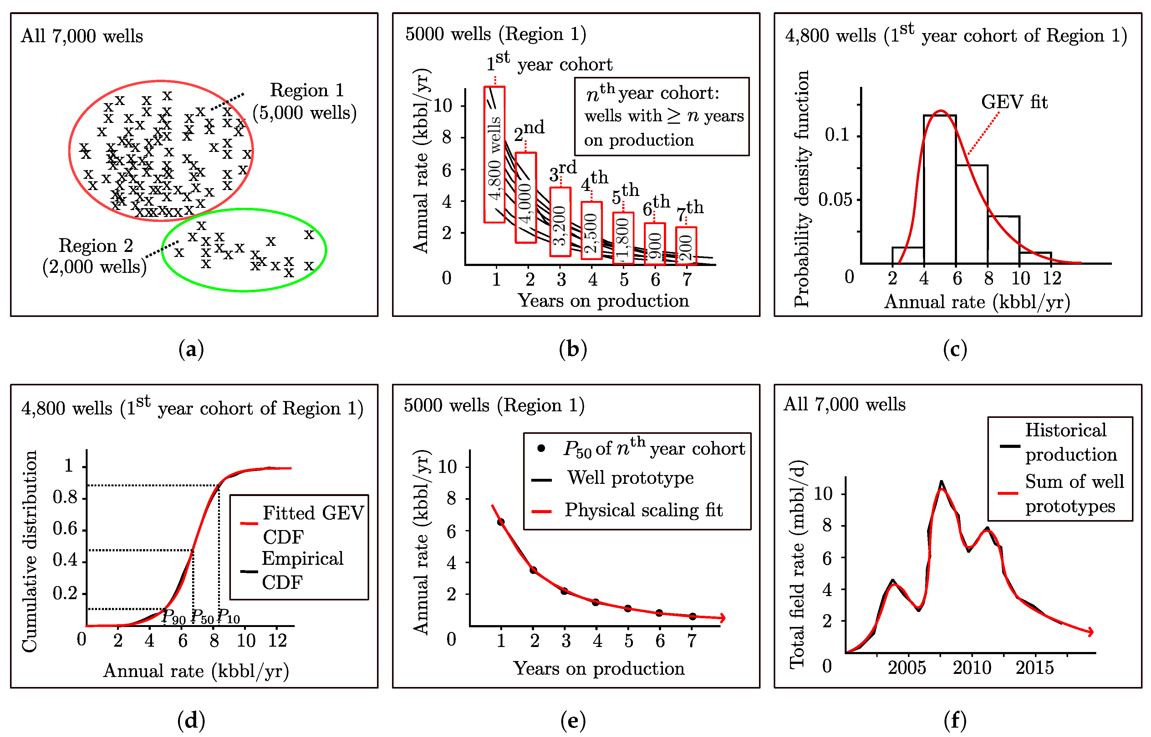
The procedure of arriving at the Generalized Extreme Value (GEV) well prototypes in a given shale play. (a) Define static regions in which oil production is statistically uniform. (b) For each region, gather the dynamic cohorts of wells with ≥i years on production, i = 1, 2, 3, .... (c) Fit GEV probability density function (PDF) to each well cohort. (d) From the corresponding cumulative distribution function (CDF) pick the P10, P50, and P90 values for each cohort. (e) Construct time-lapse P50 well prototype for each region, by connecting all P50 values of all cohorts. (f) Time-shift and superpose the GEV well prototypes to match past production. Reproduced from our previous work [21].
Figure 3.
The procedure of arriving at the Generalized Extreme Value (GEV) well prototypes in a given shale play. (a) Define static regions in which oil production is statistically uniform. (b) For each region, gather the dynamic cohorts of wells with ≥i years on production, i = 1, 2, 3, .... (c) Fit GEV probability density function (PDF) to each well cohort. (d) From the corresponding cumulative distribution function (CDF) pick the P10, P50, and P90 values for each cohort. (e) Construct time-lapse P50 well prototype for each region, by connecting all P50 values of all cohorts. (f) Time-shift and superpose the GEV well prototypes to match past production. Reproduced from our previous work [21].

Figure 4.
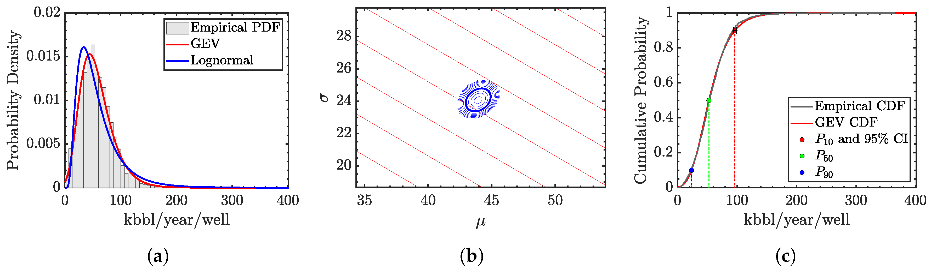
Distribution of oil production rates for 2540 horizontal wells with one year on production, completed between the year 2000 and 2012 in the Middle Bakken noncore area. (a) GEV PDF: ξ = −0.0274, μ = 43.9421, σ = 24.0635. (b) Maximum Likelihood Estimate, 95% confidence interval (CI) for μ and σ. (c) GEV CDF with the 95% CI on the residual for the P10 well.
Figure 4.
Distribution of oil production rates for 2540 horizontal wells with one year on production, completed between the year 2000 and 2012 in the Middle Bakken noncore area. (a) GEV PDF: ξ = −0.0274, μ = 43.9421, σ = 24.0635. (b) Maximum Likelihood Estimate, 95% confidence interval (CI) for μ and σ. (c) GEV CDF with the 95% CI on the residual for the P10 well.

Figure 5.
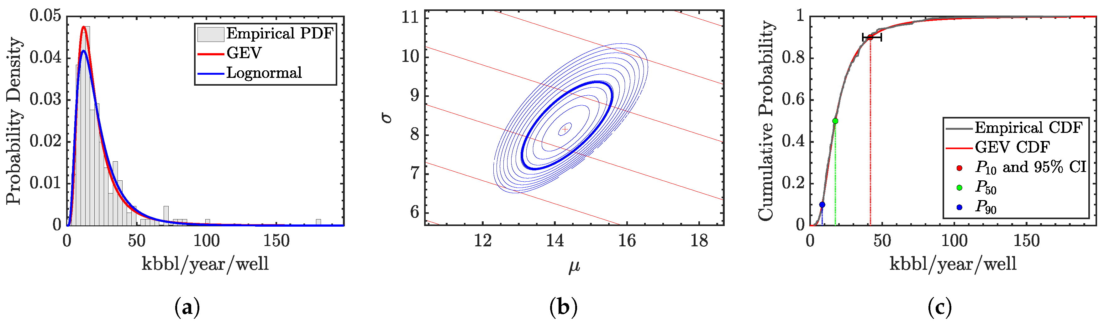
Distribution of oil production rates for 197 horizontal wells with seven years on production, completed between the year 2000 and 2012 in the Three Forks core area. (a) GEV PDF: ξ = 0.3368, μ = 14.2825, σ = 8.1499. (b) Maximum Likelihood Estimate, 95% confidence interval (CI) for μ and σ. (c) GEV CDF with the 95% CI on the residual for the P10 well.
Figure 5.
Distribution of oil production rates for 197 horizontal wells with seven years on production, completed between the year 2000 and 2012 in the Three Forks core area. (a) GEV PDF: ξ = 0.3368, μ = 14.2825, σ = 8.1499. (b) Maximum Likelihood Estimate, 95% confidence interval (CI) for μ and σ. (c) GEV CDF with the 95% CI on the residual for the P10 well.

Figure 6.
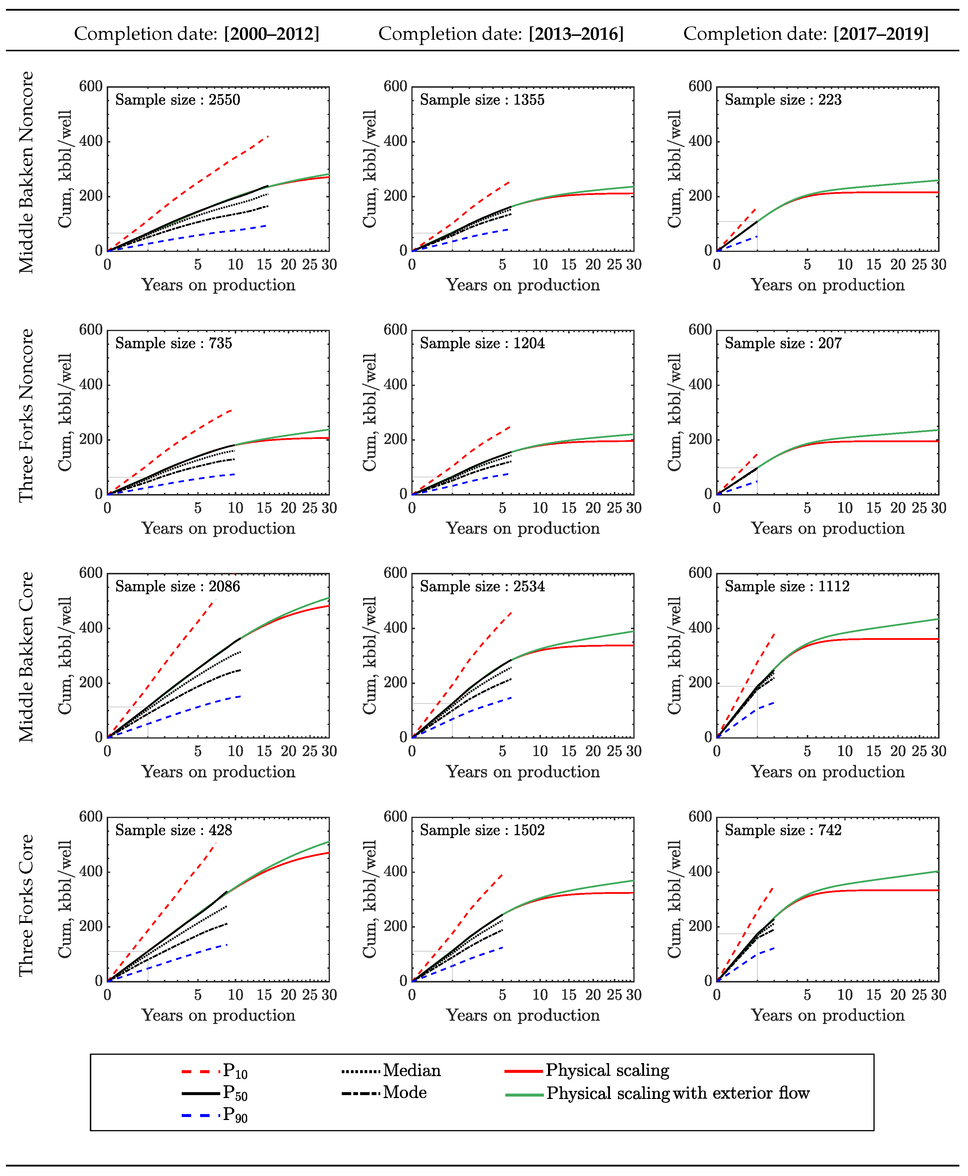
Average wells in 12 regions in the Middle Bakken and Three Forks. These wells are located in both the core and noncore areas and have three different completion periods, (2000–2012), (2013–2016) and (2017–2019). Each year in the past, every average well traces the expected values of the Generalized Extreme Value (GEV) distributions of all active horizontal wells in each well cohort, which have at least 1, 2, ..., 15 years on production. The dashed lines labeled and denote wells whose cumulative production is exceeded by 10% and 90% of wells in each region. The red and green lines are the physics-based scaling curves that match each average well, respectively, with and without exterior flow during late time production. In general, ultimate oil recovery from the core areas is higher than that from the noncore ones. The Middle Bakken wells are slightly more productive than the Three Forks wells. The newly completed wells have much higher initial oil production but they decline faster, resulting in more or less the same ultimate recovery as older wells.
Figure 6.
Average wells in 12 regions in the Middle Bakken and Three Forks. These wells are located in both the core and noncore areas and have three different completion periods, (2000–2012), (2013–2016) and (2017–2019). Each year in the past, every average well traces the expected values of the Generalized Extreme Value (GEV) distributions of all active horizontal wells in each well cohort, which have at least 1, 2, ..., 15 years on production. The dashed lines labeled and denote wells whose cumulative production is exceeded by 10% and 90% of wells in each region. The red and green lines are the physics-based scaling curves that match each average well, respectively, with and without exterior flow during late time production. In general, ultimate oil recovery from the core areas is higher than that from the noncore ones. The Middle Bakken wells are slightly more productive than the Three Forks wells. The newly completed wells have much higher initial oil production but they decline faster, resulting in more or less the same ultimate recovery as older wells.

Figure 7.
The actual and forecasted total field rate (a) and cumulative oil (b) in the Bakken shale. Total field cumulative production curves were obtained by stacking calendar-shifted average wells. Total production rates were obtained by differencing cumulative production. The red and green curves are the physical scaling forecasts with and without exterior flow, while the black line shows the historical production from the existing 14,678 wells. The red physical scaling gives the lower bound of EUR estimate with about 4.5 billion bbl by 2050. Assuming reasonable exterior flow, EUR prediction becomes slightly more than 5 billion bbl.

Figure 8.
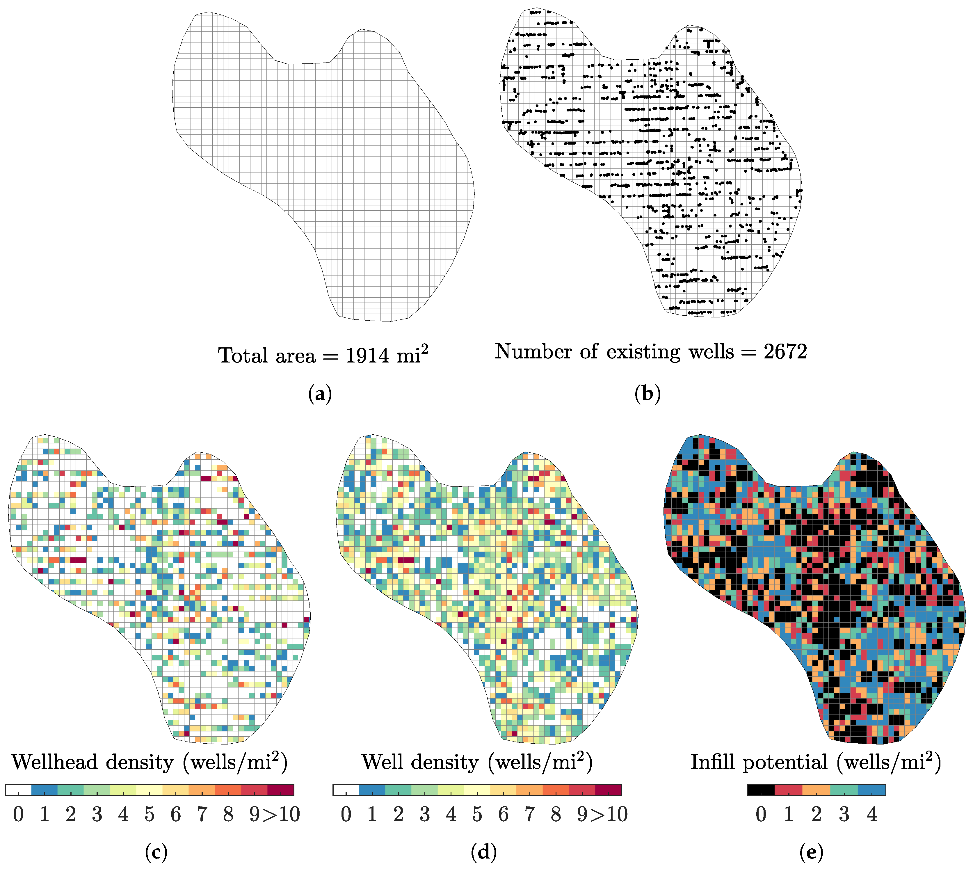
A procedure to calculate infill well potential for each part of the Bakken play. This figure shows only the Three Forks core area. For other areas and reservoirs, please see the Supporting Online Materials. The procedure is as follows: (a) Create a one-square-mile fishnet inside the boundary of each area. In this case, there are 1914 grid squares that translate into the total area of 1914 mi2. (b) Search all existing wells located inside the boundary. The black dots show the surface locations of 2672 existing wells in Three Forks core area. (c) Calculate wellhead density by counting the number of wells on each of the one-square-mile squares. This map is not the real well density map, because it only shows the wellhead density. (d) Calculate an approximate well density map from wellhead density map. The algorithm is as follows: (1) For each well, record its lateral length and calculate the number of squares, n, intercepted by the lateral. For example, a 5000 ft lateral will occupy one square and a 10,000 ft lateral will occupy two squares because one mile is 5280 ft. (2) Search for the least occupied n squares in all possible directions (i.e., north, northeast, east, southeast, south, southwest, west and northwest). (3) Increase the value of well density by 1 well/mi2 for every least dense square found. (4) Repeat the process until all wells in the area of interest are exhausted. (e) Calculate an infill potential map by subtracting the calculated well density from the maximum number of wells, Nmax (e.g., Nmax = 4 wells/mi2 to avoid frac hits). The summation of all values in the map is the infill potential for the one-square-mile grid. In this case, we obtain 3650 wells. As most wells have 10,000 ft laterals and occupy two one-square-mile squares, we divide 3650 by 2 to obtain 1825 infill potential wells in the Three Forks core area.
Figure 8.
A procedure to calculate infill well potential for each part of the Bakken play. This figure shows only the Three Forks core area. For other areas and reservoirs, please see the Supporting Online Materials. The procedure is as follows: (a) Create a one-square-mile fishnet inside the boundary of each area. In this case, there are 1914 grid squares that translate into the total area of 1914 mi2. (b) Search all existing wells located inside the boundary. The black dots show the surface locations of 2672 existing wells in Three Forks core area. (c) Calculate wellhead density by counting the number of wells on each of the one-square-mile squares. This map is not the real well density map, because it only shows the wellhead density. (d) Calculate an approximate well density map from wellhead density map. The algorithm is as follows: (1) For each well, record its lateral length and calculate the number of squares, n, intercepted by the lateral. For example, a 5000 ft lateral will occupy one square and a 10,000 ft lateral will occupy two squares because one mile is 5280 ft. (2) Search for the least occupied n squares in all possible directions (i.e., north, northeast, east, southeast, south, southwest, west and northwest). (3) Increase the value of well density by 1 well/mi2 for every least dense square found. (4) Repeat the process until all wells in the area of interest are exhausted. (e) Calculate an infill potential map by subtracting the calculated well density from the maximum number of wells, Nmax (e.g., Nmax = 4 wells/mi2 to avoid frac hits). The summation of all values in the map is the infill potential for the one-square-mile grid. In this case, we obtain 3650 wells. As most wells have 10,000 ft laterals and occupy two one-square-mile squares, we divide 3650 by 2 to obtain 1825 infill potential wells in the Three Forks core area.

Figure 9.
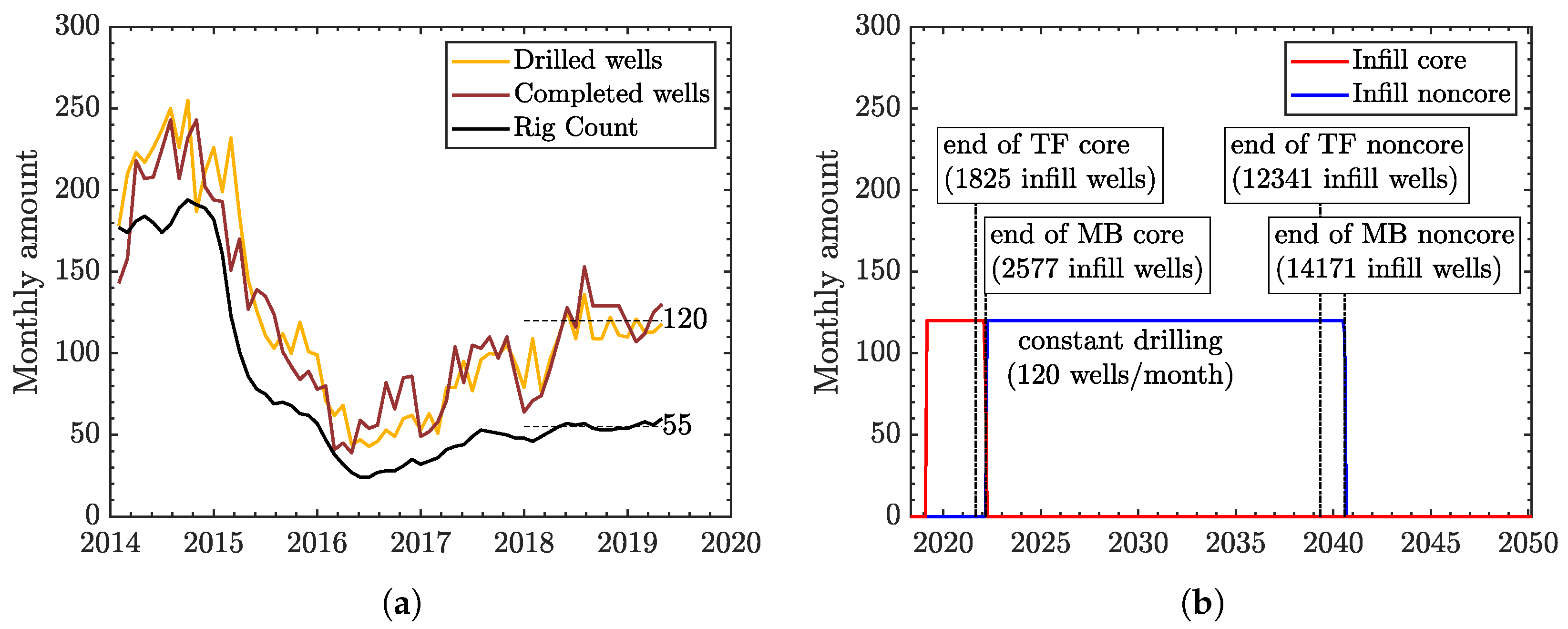
(a) The number of drilled wells, completed wells and rig count per month for the Bakken play from the U.S. Energy Information Administration (EIA). The drilled and completed wells are almost the same for each month and are strongly correlated with the number of rigs available. These data reveal an increase in drilling efficiency. In 2015, one rig could drill about 1.2 wells per month, while in 2019 so far, one rig could drill two wells per month. The current drilling rate is constant at about 120 wells/month. (b) A future drilling scenario for the Bakken region up to 2041. The plan is to continue at the current drilling rate of 120 wells/month for both core and noncore areas. The numbers of wells to be infilled in each region were previously calculated using the procedure detailed in Figure 8. The results show that the core areas will be fully drilled by mid 2022, leaving the less productive noncore areas for infilling until 2041.
Figure 9.
(a) The number of drilled wells, completed wells and rig count per month for the Bakken play from the U.S. Energy Information Administration (EIA). The drilled and completed wells are almost the same for each month and are strongly correlated with the number of rigs available. These data reveal an increase in drilling efficiency. In 2015, one rig could drill about 1.2 wells per month, while in 2019 so far, one rig could drill two wells per month. The current drilling rate is constant at about 120 wells/month. (b) A future drilling scenario for the Bakken region up to 2041. The plan is to continue at the current drilling rate of 120 wells/month for both core and noncore areas. The numbers of wells to be infilled in each region were previously calculated using the procedure detailed in Figure 8. The results show that the core areas will be fully drilled by mid 2022, leaving the less productive noncore areas for infilling until 2041.

Figure 10.
The forecasted total field rate (a) and cumulative oil (b) for Bakken based on the drilling scenario in Figure 9b. Since we plan to infill the core areas first, the field oil rate will reach the all-time production peak of about 1.6 million bbl/d by mid 2022, leaving no ‘sweet spots’ in the core areas. The continuous infill of the less productive wells in the noncore areas will decline the production to a plateau of 1 million bbl/d. After 2041, no more drilling locations will be left in the Bakken region and the oil rate will steeply decline to half a million bbl/d by 2042 and 0.2 million bbl/d by 2050. Ultimately, the 14,898 existing wells will give an EUR of 5 billion bbl. By adding 4402 wells in the core areas, EUR will increase to 7 billion bbl. By adding another 26,512 wells in the noncore areas, EUR will increase to 13 billion bbl.

Table 1.
Static regions for the Bakken shale play.
| Well | Reservoir | Area | Completion | Sample |
|---|---|---|---|---|
| Sample | Date | Size | ||
| 1 | Middle Bakken | Noncore | 2000–2012 | 2550 |
| 2 | Middle Bakken | Noncore | 2013–2016 | 1355 |
| 3 | Middle Bakken | Noncore | 2017–2019 | 223 |
| 4 | Three Forks | Noncore | 2000–2012 | 735 |
| 5 | Three Forks | Noncore | 2013–2016 | 1204 |
| 6 | Three Forks | Noncore | 2017–2019 | 207 |
| 7 | Middle Bakken | Core | 2000–2012 | 2086 |
| 8 | Middle Bakken | Core | 2013–2016 | 2534 |
| 9 | Middle Bakken | Core | 2017–2019 | 1112 |
| 10 | Three Forks | Core | 2000–2012 | 428 |
| 11 | Three Forks | Core | 2013–2016 | 1502 |
| 12 | Three Forks | Core | 2017–2019 | 742 |
| TOTAL | 14,678 | |||
Table 2.
Scaling parameters for an average well in the Bakken regions.
| Well Sample | Physical Scaling | Physical Scaling with Exterior Flow | ||||||
|---|---|---|---|---|---|---|---|---|
| Shift Years | Years | kbbl/Well | EUR kbbl/Well | Years | a | EUR kbbl/Well | ||
| Middle Bakken noncore [2000–2012] | 0.25 | 24.5 | 454.3 | 271.1 | 19.9 | 286.7 | 0.050 | 282.2 |
| Middle Bakken noncore [2013–2016] | 0.00 | 11.8 | 341.3 | 211.7 | 10.9 | 267.2 | 0.026 | 236.4 |
| Middle Bakken noncore [2017–2019] | 0.00 | 5.0 | 346.9 | 215.5 | 5.0 | 306.6 | 0.015 | 259.5 |
| Three Forks noncore [2000–2012] | 0.15 | 13.3 | 288.4 | 207.5 | 10.7 | 181.2 | 0.058 | 238.3 |
| Three Forks noncore [2013–2016] | 0.00 | 10.8 | 271.9 | 196.1 | 9.9 | 212.4 | 0.030 | 221.1 |
| Three Forks noncore [2017–2019] | 0.00 | 5.0 | 270.8 | 195.4 | 5.0 | 238.4 | 0.018 | 236.5 |
| Middle Bakken core [2000–2012] | 0.20 | 25.0 | 810.8 | 482.5 | 22.6 | 536.3 | 0.050 | 512.2 |
| Middle Bakken core [2013–2016] | 0.00 | 9.1 | 543.8 | 337.7 | 8.2 | 420.7 | 0.026 | 389.7 |
| Middle Bakken core [2017–2019] | 0.00 | 5.0 | 581.9 | 361.5 | 5.0 | 513.6 | 0.015 | 434.6 |
| Three Forks core [2000–2012] | 0.27 | 25.0 | 681.1 | 470.9 | 25.0 | 473.4 | 0.058 | 511.6 |
| Three Forks core [2013–2016] | 0.00 | 10.3 | 450.1 | 324.6 | 9.6 | 353.1 | 0.030 | 369.7 |
| Three Forks core [2017–2019] | 0.00 | 5.0 | 462.8 | 334.0 | 5.0 | 406.9 | 0.018 | 403.5 |
Table 3.
Infill potential for Bakken region.
| Reservoir | Region | Total Area | Existing | Infill |
|---|---|---|---|---|
| Type | sq Miles | Wells | Potential | |
| Middle Bakken | Noncore | 8534.5 | 4128 | 14,171 * |
| Three Forks | Noncore | 6905.9 | 2146 | 12,341 * |
| Middle Bakken | Core | 3382.5 | 5732 | 2577 |
| Three Forks | Core | 1914.1 | 2672 | 1825 |
| TOTAL | 20,737 | 14678 | 30,914 | |
* Given the low reservoir quality in noncore areas, our infill potentials there are probably too high.
© 2019 by the authors. Licensee MDPI, Basel, Switzerland. This article is an open access article distributed under the terms and conditions of the Creative Commons Attribution (CC BY) license (http://creativecommons.org/licenses/by/4.0/).
Share and Cite
MDPI and ACS Style
Saputra, W.; Kirati, W.; Patzek, T. Generalized Extreme Value Statistics, Physical Scaling and Forecasts of Oil Production in the Bakken Shale. Energies 2019, 12, 3641. https://doi.org/10.3390/en12193641
AMA Style
Saputra W, Kirati W, Patzek T. Generalized Extreme Value Statistics, Physical Scaling and Forecasts of Oil Production in the Bakken Shale. Energies. 2019; 12(19):3641. https://doi.org/10.3390/en12193641
Chicago/Turabian StyleSaputra, Wardana, Wissem Kirati, and Tadeusz Patzek. 2019. "Generalized Extreme Value Statistics, Physical Scaling and Forecasts of Oil Production in the Bakken Shale" Energies 12, no. 19: 3641. https://doi.org/10.3390/en12193641
Note that from the first issue of 2016, this journal uses article numbers instead of page numbers. See further details here.