2.1 A priori fluxes and uncertainties

The prior estimates for net ecosystem production (NEP = photosynthesis − respiration) and fire emissions (wildfires, biomass burning, and biofuel burning) come from the Carnegie-Ames-Stanford-Approach (CASA) biogeochemical model coupled to version 3 of the Global Fire Emissions Database (GFED3; Randerson et al., 1996; van der Werf et al., 2006, 2010). CASA-GFED is driven with data on fraction of absorbed photosynthetically active radiation (FPAR) derived from the AVHRR satellite series (Pinzon and Tucker, 2014; Los et al., 2000), burned area from MODIS (Giglio et al., 2010), and meteorology (precipitation, temperature, and solar radiation) from the Modern-Era Retrospective Analysis for Research and Applications (MERRA; Rienecker et al., 2011). CASA-GFED fluxes are generated at 0.5^∘ × 0.5^∘ resolution. For use in the atmospheric transport model, monthly fluxes are downscaled to 3-hourly values using solar radiation and temperature (Olsen and Randerson, 2004) along with MODIS 8-day satellite fire detections (Giglio et al., 2006). In general, the biosphere is close to neutral in the CASA-GFED simulation, i.e., there is no long-term net sink although there can be interannual variations in the balance between uptake and release. In the version of CASA used here, a sink of ∼ 100 Tg C yr⁻¹ is induced by crop harvest in the US Midwest that is prescribed based on National Agriculture Statistics Service data on crop area and harvest. Although respiration of the harvested products is neglected, the underestimate of emissions that is implied is geographically dispersed and in principle correctable by the inversion.

For air–sea CO₂ exchange, monthly, climatological, measurement-based fluxes are taken from Takahashi et al. (2009) for the reference year 2000 on a 4^∘ × 5^∘ lat/long grid. In contrast to the CASA-GFED flux being close to neutral on a global basis, the prior ocean flux forms a net sink of 1.4 Pg C yr⁻¹. For fossil CO₂, 1^∘ × 1^∘, monthly and interannually varying emissions are taken from the Carbon Dioxide Information Analysis Center (CDIAC) inventory (Andres et al., 2012). This includes CO₂ from cement production but not international shipping and aviation emissions. Oxidation of reduced carbon-containing gases from fossil fuels in the atmosphere (∼ 5% of the emissions; Nassar et al., 2010) is neglected, and the entire amount of the emissions is released as CO₂ at the surface. Similarly, CO₂ from oxidation of biogenic and biomass burning gases is neglected. Together these oxidation sources are estimated to be ∼ 1 Pg C yr⁻¹ (for year 2006; Nassar et al., 2010).

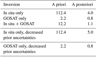
Table 1Inversion prior and posterior fluxes and uncertainties (Unc.) aggregated to TransCom 3 regions, June 2009–May 2010.

^a Fluxes in table, in Pg C, include fires but not fossil emissions. ^b U.R. is an abbreviation for uncertainty reduction.

Download Print Version | Download XLSX

A priori flux uncertainties are derived from those assumed in the TC3 studies (Table 1), rescaled to our smaller regions and shorter periods with the same approach as Feng et al. (2009). The uncertainties are large enough to accommodate possible biases, e.g., the neutral biosphere rather than a sizable net land sink as suggested by the literature. A priori spatial and temporal error correlations are neglected in our standard inversions. The neglect of a priori spatial error correlations is justified by the size of our flux optimization regions, with dimensions on the order of one thousand to several thousand kilometers, likely greater than the error correlation lengths for our 2^∘ × 2.5^∘ grid-level fluxes. For example, Chevallier et al. (2012) estimated a correlation e-folding length of ∼ 500 km for a grid size close to ours of 300 km × 300 km based on comparison of a terrestrial ecosystem model with global flux tower data.

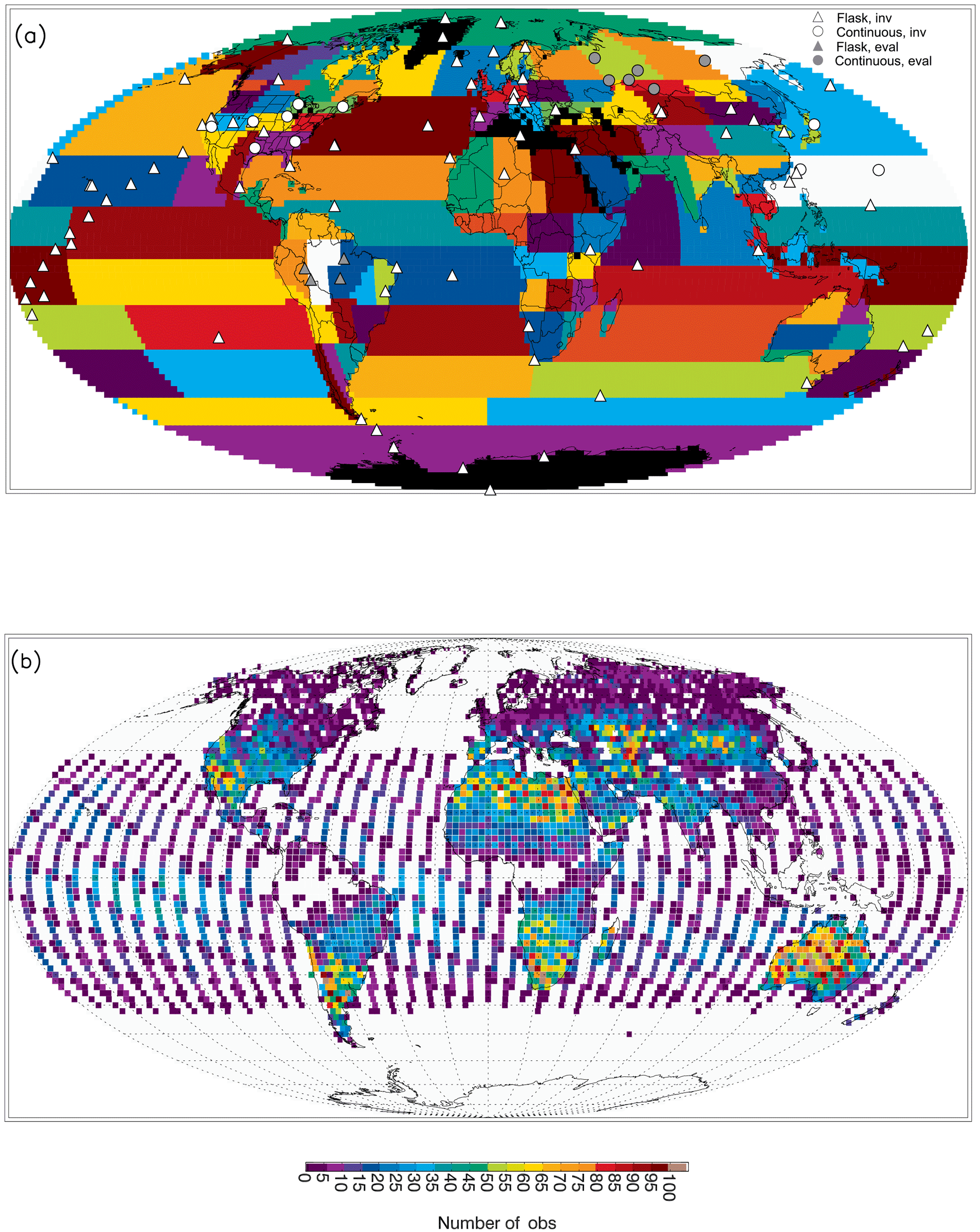
Figure 1Locations of (a) in situ observation sites and (b) GOSAT XCO₂ observations used in the inversions. Also shown in (a) are the 108 flux regions. Flask and continuous measurement sites in (a) are represented by different symbols, and sites used in inversions and in their evaluation are represented by different colors. Observations in (b) correspond to the ACOS B3.4 retrieval, are filtered and averaged over each hour and 2^∘ × 2.5^∘ PCTM model grid column, and are shown for June 2009–May 2010.

Download

2.2 Observations and uncertainties

For constraining fluxes at relatively high temporal resolution, observations are chosen that consist of discrete whole-air samples collected in glass flasks approximately weekly and continuous in situ tall tower measurements of CO₂ mole fraction from the NOAA ESRL Carbon Cycle Cooperative Global Air Sampling Network (Dlugokencky et al., 2013; Andrews et al., 2009) supplemented with continuous ground-based measurements at three sites in East Asia from the Japan Meteorological Agency (JMA) network (http://ds.data.jma.go.jp/gmd/wdcgg/cgi-bin/wdcgg/catalogue.cgi, last access: 14 March 2013; Tsutsumi et al., 2006). Both data sets are calibrated to the WMO-X2007 scale. In the present study, these data sets are referred to collectively as “in situ” observations. The 87 sites (Fig. 1a; Table S1) are chosen based on data availability for the analysis period, March 2009–September 2010. Individual flask-air observations are used in the inversions (with the average taken where there are multiple measurements at a particular hour – up to two pairs of duplicate flasks), and for the continuous measurements, afternoon averages are used (between 12:00 and 17:00 LT, local time), avoiding the difficulty of simulating the effects of shallow nighttime boundary layers. For the towers, data from the highest level only is used. We apply minimal filtering of the data. For the NOAA data sets, we exclude only the flask samples or 30-second-average continuous data with “rejection” flags, retaining data with “selection” flags (NOAA uses statistical filters and other information such as wind direction to flag data that are likely valid but do not meet certain criteria such as being representative of well-mixed, background conditions), since the reasonably high-resolution transport model used here (Sect. 2.3) captures much of the variability in the observations beyond background levels. Furthermore, observations strongly influenced by local fluxes are typically assigned larger uncertainties by our scheme (described below), and therefore have less weight in the inversion. For the JMA data, we omit only the hourly data with flag = 0, meaning the number of samples is below a certain level, the standard deviation is high, and there is a large discrepancy with one or both adjacent hourly values. Although some of the observation sites used in our inversion are located close to each other, there is never any exact overlap in grid box (altitude and/or longitude–latitude) or in time. Thus, all of those sites are kept for the inversions, with observations at each site and day treated as independent (i.e., neglecting error correlations).

Table 2Normalized cost function values for the inversions.

Download Print Version | Download XLSX

We estimate the uncertainties for the flask-air observations as the root sum square (RSS) of two components: (1) the standard deviation of the observations from multiple flasks within an hour or 0.3 ppm if there is only one sample, and (2) a simple estimate of the model transport and representation error. The transport and representation error estimation is similar to that of the NOAA CarbonTracker (CT) CO₂ data assimilation system (prior to the CT 2015 version; Peters et al., 2007; http://carbontracker.noaa.gov, last access: 19 January 2018), whereby a fixed “model-data mismatch” is assigned based on the type of site, e.g., marine, coastal, continental, or polluted, ranging from 0.4 to 4 ppm (Table S1). For the continuous measurements, we take the RSS of two uncertainty components: (1) the afternoon root mean square (RMS) of the uncertainties in the 30 s (NOAA) or hourly (JMA) observations reported by the data providers, divided by the square root of the number of observations, N, and (2) the standard error of all the 30 s or hourly mole fractions within an afternoon period. This represents an attempt to account for instrument error as well as transport and representation error. In addition, based on initial inversion results, we enlarged all in situ total observation uncertainties by a factor of 2 (mean site values in Table S1 in the Supplement) to lower the normalized posterior cost function value (defined in Sect. 2.4) closer to 1 as appropriate for the chi-squared (χ²) distribution (the final value of which is shown in Table 2). (Another test showed that further enlargement of the uncertainties to 3 times the original values, while lowering the cost function value further, does not substantially change the posterior fluxes overall.)

GOSAT measures reflected sunlight in a sun-synchronous orbit with a 3-day repeat cycle and a 10.5 km diameter footprint when in nadir mode (Yokota et al., 2009). The spacing between soundings is ∼ 250 km along-track and ∼ 160 km or ∼ 260 km cross-track (for 5-point or 3-point sampling before or after August 2010). We use the ACOS B3.4 near infrared (NIR) retrieval of column-average CO₂ dry air mole fraction (XCO₂), with data from June 2009 onward (O'Dell et al., 2012; Osterman et al., 2013). Filtered and bias-corrected land nadir, including high (H) gain and medium (M) gain, and ocean glint data are provided. Three truth metrics were used together to correct biases (separately for H gain, M gain, and ocean glint) (Osterman et al., 2013; Lindqvist et al., 2015; Kulawik et al., 2016): (1) an ensemble of transport model simulations optimized against in situ observations, (2) coincident ground-based column observations from the Total Carbon Column Observing Network (TCCON), which are calibrated to aircraft in situ profiles linked to the WMO scale (Wunch et al., 2011), and (3) the assumption that CO₂ mole fraction ought to exhibit little spatiotemporal variability in the Southern Hemisphere mid-latitudes, other than a seasonal cycle and long-term trend. For our inversions, we use the average of all GOSAT observations falling within a given 2^∘ latitude × 2.5^∘ longitude transport model column in a given hour. Figure 1b shows the frequency of the ACOS GOSAT observations across the model grid.

The values assumed for the GOSAT uncertainties are based in part on the retrieval uncertainties provided with the ACOS data set. Following guidance from the data providers, these are inflated by a factor of 2 over land and 1.25 over ocean for more realistic estimates of the uncertainties (Christopher O'Dell, personal communication, 2013); Kulawik et al. (2016) recommended an overall scale factor of 1.9 for the similar ACOS B3.5 data set. In the case of multiple observations within a model grid, we estimate the overall uncertainty as the RMS of the uncertainties in the individual observations, divided by the square root of N. Final uncertainty values are in the range of 0.31–3.20 ppm over land and 0.26–1.94 ppm over ocean, with corresponding means of 1.48 and 0.77 ppm. Error correlations between observations in different model grids and at different hours are neglected.

Inversions are conducted using different combinations of data, including the in situ data (“in situ only”), the GOSAT data (“GOSAT only”), and both (“in situ + GOSAT”).

We use several additional data sets for independent evaluation of the inversion results. Aircraft measurements from the HIAPER Pole-to-Pole Observations (HIPPO) campaign consist of vertical profiles of climate-relevant gases and aerosols from the surface to as high as the lower stratosphere, spanning a wide range of latitudes mostly over the Pacific region (Wofsy et al., 2011). Five missions were conducted during different seasons during 2009–2011, with two of the missions overlapping with our analysis period. We use the “best available” CO₂ values derived from multiple measurement systems from the merged 10 s data product (Wofsy et al., 2012). Another data set, the “Amazonica” aircraft measurements over the Amazon basin, is useful for evaluating inversion performance over tropical land. These measurements consist of profiles of several gases including CO₂ determined from flask samples from just above the forest canopy to 4.4 km altitude over four sites across the Brazilian Amazon starting in 2010, taken approximately biweekly (Gatti et al., 2014, 2016). Finally, the Japan–Russia Siberian Tall Tower Inland Observation Network (JR-STATION) of towers provides continuous in situ measurements of CO₂ and CH₄ over different ecosystem types across Siberia beginning in 2002 (Sasakawa et al., 2010, 2013). The JR-STATION data have been used in combination with other in situ observations in CO₂ flux inversions (Saeki et al., 2013b; Kim et al., 2017).

2.3 Atmospheric transport model and model sampling

We use the Parameterized Chemistry and Transport Model (PCTM; Kawa et al., 2004), with meteorology from the NASA Global Modeling and Assimilation Office (GMAO) MERRA reanalysis (Rienecker et al., 2011). For this analysis, PCTM was run at a resolution of 2^∘ latitude × 2.5^∘ longitude and 56 hybrid terrain-following levels up to 0.4 hPa, and hourly temporal resolution. A “pressure fixer” scheme has been implemented to ensure tracer mass conservation, the lack of which can be a significant problem with assimilated winds (Kawa et al., 2004). Evaluation of PCTM over the years has shown it to be a reliable tool for carbon cycle studies. For example, Kawa et al. (2004) showed that the SF₆ distribution from PCTM was consistent with that of observations and of the models in TransCom 2, suggesting that the interhemispheric and vertical transport were reasonable. PCTM performed well in boundary layer turbulent mixing compared to most of the other models in a TransCom investigation of the CO₂ diurnal cycle (Law et al., 2008). The TransCom-CH₄ intercomparison (Patra et al., 2011) showed that a more recent version of PCTM performed very well relative to observations in its interhemispheric gradients of SF₆, CH₃CCl₃, and CH₄ and in its interhemispheric exchange time, and follow-on studies (Saito et al., 2013; Belikov et al., 2013) demonstrated through evaluation against observed CH₄ and ²²²Rn that the convective vertical mixing in PCTM was satisfactory overall.

Offshore prior terrestrial biospheric and fossil fluxes are redistributed to the nearest onshore grid cells in the model grid to counteract diffusion caused by our regridding the original fluxes to the coarser 2^∘ × 2.5^∘ resolution, as recommended in the TC3 protocol (Gurney et al., 2000).

The model is initialized with a concentration field appropriate for 22 March 2009 from a multi-year PCTM run with prior fluxes. The initial conditions are optimized in the inversions, as described in Sect. 2.4.

PCTM is sampled at grid cells containing in situ observation sites or GOSAT soundings, at the hours corresponding to the observations. To mimic the sampling protocol for coastal flask sites, which favors clean, onshore wind conditions, the model is sampled at the neighboring offshore grid cell if the cell containing the site is considered land according to a land/ocean mask. For in situ sites in general, an appropriate vertical level as well as horizontal location is selected. Specifically, the model CO₂ profile is interpolated to a level corresponding, on average, to the altitude above sea level of the observation site. This procedure is relevant primarily for mountain sites and tall towers as well as aircraft samples; the lowest model layer (with a thickness of ∼ 100 m on average) was used for most other sites.

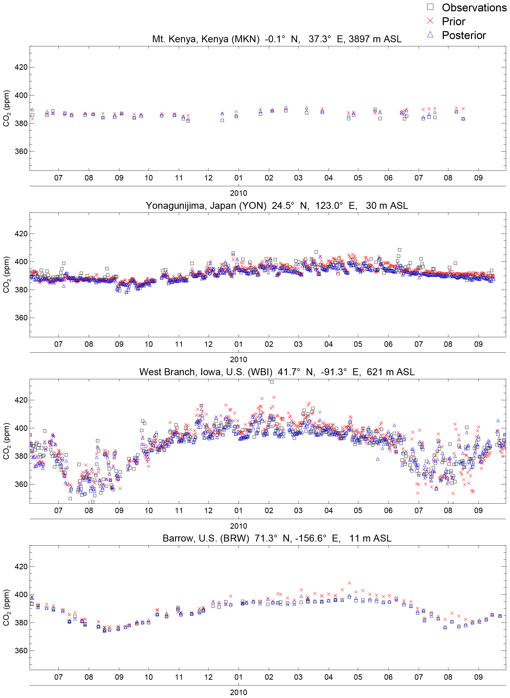
Figure 2Comparison of model and observed time series of CO₂ mole fractions at selected surface sites. Posterior mole fractions are for the in situ only inversion. Sites are arranged from south to north. The elevation for the West Branch, Iowa (WBI) site includes the intake height on the tower.

Download

Model columns are weighted using ACOS column averaging kernels, as in the following (Eq. 15 from Connor et al., 2008):

where $X_{{\mathrm{CO}}_{\mathrm{2}}}^{\text{m}}$ ($X_{{\mathrm{CO}}_{\mathrm{2}}}^{\text{a}})$ refers to the model (ACOS a priori) column average mole fraction, h is the pressure weighting function, ${\mathit{a}}_{{\mathrm{CO}}_{\mathrm{2}}}$ is the column averaging kernel, x refers to a CO₂ profile, and j is the level index.

Time series of model and observed mole fractions at selected flask and continuous sites spanning a range of latitudes, longitudes, elevations, and proximity to major fluxes are shown for the prior and for the in situ only inversion in Fig. 2. The prior model as well as the in situ inversion captures much of the observed synoptic-scale variability. This suggests that the PCTM transport is reasonably accurate, consistent with the findings of Parazoo et al. (2008) and Law et al. (2008).

2.4 Inversion approach

The batch, Bayesian synthesis inversion approach optimizes in a single step the agreement between model and observed CO₂ mole fractions and between a priori and a posteriori flux estimates in a least-squares manner (e.g., Enting et al., 1995). As in the paper by Baker et al. (2006), the cost function minimized in this approach can be expressed as

where c_obs−c_fwd are mismatches between the observations and the mole fractions produced by the prior fluxes, H is the Jacobian matrix relating model mole fractions at the observation locations to regional flux adjustments x (note that x is used differently here than in Eq. 1). R is the covariance matrix for the errors in c_obs−c_fwd, x₀ is an a priori estimate of the flux adjustments, and P₀ is the covariance matrix for the errors in x₀. The solution for the a posteriori flux adjustments, $\widehat{\mathit{x}}$, is

and the a posteriori error covariance matrix is given by

Importantly, the posterior uncertainties do not account for possible biases, given that the Bayesian inversion framework adopted here, as in other CO₂ studies, assumes Gaussian error distributions with no bias (observation, transport, prior, etc.).

This study focuses on the variability in natural fluxes (terrestrial NEP and ocean), and thus considers adjustments to those fluxes only, assuming the prior estimates for the fossil and fire fluxes are correct. This is commonly done in CO₂ inversion studies (e.g., Gurney et al., 2002; Peters et al., 2007; Basu et al., 2013), with the rationale that the anthropogenic emissions are relatively well known, at least at the coarse spatial scales of most global inversions. In our inversion, flux adjustments are solved for at a resolution of 8 days and for each of the 108 regions that are modified from the 144 regions of the Feng et al. (2009) inversion (Fig. 1a), which are in turn subdivided from the TC3 regions. (The choice of an 8-day flux interval is based on data considerations, e.g., the quasi-weekly frequency of the flask measurements and reasonable sampling by GOSAT.) This is a significantly higher resolution than the monthly intervals and 22 (47) regions in the previous batch inversions of TC3 (Butler et al., 2010), which allows us to take advantage of the relatively high density of the GOSAT observations. One of our regions consists of low-flux areas (e.g., Greenland, Antarctica) as well as small offshore areas that contain non-zero terrestrial biospheric fluxes but do not fit into any of the TC3-based land regions, similar to what was done by Feng et al. (2009). We also created a region that includes areas with non-zero oceanic fluxes that do not fit into any of the TC3-based ocean regions according to our gridding scheme.

Grid-scale spatial patterns are imposed in our flux adjustments based on the natural fluxes, similar to TC3 and Butler et al. (2010), except that we use patterns specific to our prior NEP or air–sea flux averaged over each particular 8-day period, rather than annual mean net primary productivity (NPP) patterns over land and spatially constant patterns over the ocean. To ensure net changes in flux are possible across each region, absolute values are used for the flux patterns. Prior values of 0 are specified for all flux adjustments.

The initial conditions (i.c.) are also optimized at the same time as the fluxes via two parameters: a scale factor to the i.c. tracer (described below) that allows for overall adjustment of spatial gradients, and a globally uniform offset. A priori uncertainties of 0.01 for the scale factor and 30 ppm for the offset are prescribed. Inversion results from March 22 through 30 April 2009 are discarded to avoid the influence of any inaccuracies in the i.c. (Our tests showed that inferred fluxes after the first two months are insensitive to the treatment of i.c. For example, for an in situ inversion in which we did not allow adjustments in the i.c. and offset parameters, 8-day average flux results are very similar to those of the baseline inversion, especially after the first two months, with a mean correlation coefficient of 0.95 from June 2009 onward across all TC3 regions and a mean difference of 0.03 Pg C yr⁻¹.) Although the GOSAT data set begins in June 2009, the observations can provide some constraint on earlier fluxes.

For generating the prior mole fractions, c_fwd, and constructing the Jacobian matrix, H, transport model runs were performed for each of the prior flux types and an i.c. tracer, as well as a run with a flux pulse (normalized to 1 Pg C yr⁻¹) for each of the 108 regions and 71 8-day periods. (The last period in 2009 is shortened to 5 days to fit cleanly within the year.) The i.c. tracer is initialized as described in Sect. 2.3 and transported without emissions or removals for the duration of the analysis period. Each flux pulse is transported for up to 13 months, after which the atmosphere is well mixed (within a range of 0.01 ppm). This procedure generated a massive amount of 3-D model output, ∼ 30 terabytes (compressed). All of the model output was then sampled at the observation locations and times.

A singular value decomposition (SVD) approach is used instead of direct computation of Eqs. (3) and (4) to obtain a stable inversion solution without any need for truncation of singular values below a certain threshold (Rayner et al., 1999). Use of the SVD technique is especially helpful in the case of the inversions using GOSAT data, since the Jacobian matrix is too large (92 762 (102 210) × 7674 for GOSAT (in situ + GOSAT)) to be successfully inverted on our system (with a single CPU).

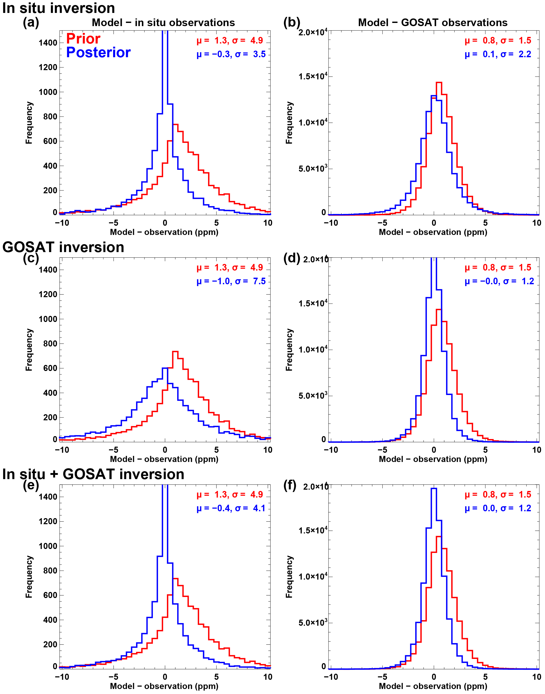
Figure 3Full comparison of model and observations. Model-observation difference histograms are shown for (a) in situ only inversion and in situ observations, (b) in situ only inversion and GOSAT observations, (c) GOSAT only inversion and in situ observations, (d) GOSAT only inversion and GOSAT observations, (e) in situ + GOSAT inversion and in situ observations, and (f) in situ + GOSAT inversion and GOSAT observations. Mean differences and standard deviations are indicated in the panels.

Download

3.1 General evaluation of inversions, including short-term flux variability

Posterior model mole fractions are closer to the assimilated observations than are the prior mole fractions for the in situ only, GOSAT only, and in situ + GOSAT inversions, as desired, as suggested by Fig. 2 and indicated by the means and standard deviations of the model-observation differences over all observations shown in Fig. 3a, d, e, and f. Comparison of posterior mole fractions with the data set not used (Fig. 3b, c), on the other hand, gives mean differences not as close to 0 as in the comparison with the assimilated data (Fig. 3d and a, respectively), and standard deviations that are larger than for the prior; this reflects the fact that the in situ and GOSAT data sets are not necessarily consistent with each other and combine to produce larger standard deviations than with the less variable prior model, which has not assimilated any data. The improved agreement between model and assimilated observations is reflected also in the cost function values before and after the inversions shown in Table 2. The minimized cost function follows a χ² distribution, and thus should have a value close to 1 (normalized by the number of observations) for a satisfactory inversion (Tarantola, 1987; Rayner et al., 1999). The posterior cost function values for all of the inversions are closer to 1 than the prior values.

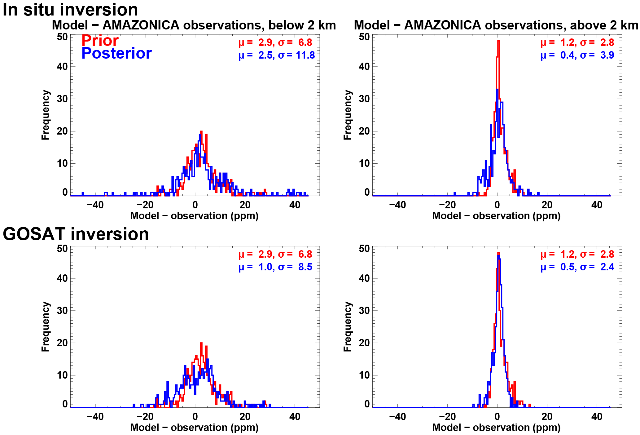
Figure 4Comparison of model and Amazon aircraft observations (Amazonica project) over the period of overlap, January–September 2010. Top two panels show model-observation difference histograms for the in situ only inversion and bottom two panels show results for the GOSAT only inversion. Comparisons are shown separately for model and data below 2 km altitude (left) and above 2 km (right). Mean differences and standard deviations are indicated in the panels.

Download

In addition to cross-evaluating the in situ only and GOSAT only inversions, we evaluate both inversions against the independent, well-calibrated Amazon aircraft data set, which samples an under-observed region with large, variable fluxes. Vertical profiles of the model and the aircraft data (Fig. S1) show that the prior mole fractions often exhibit a bias relative to the aircraft observations, especially in a boundary-layer-like structure below ∼ 2 km altitude, with the sign of the average bias varying from season to season. The in situ inversion exhibits worse agreement with the observations than the prior does more often than it is better (e.g., with a root mean square error, RMSE, that is more than 1 ppm larger in 27 of 60 cases above 2 km and in 27 cases below 2 km, and more than 1 ppm smaller in only 12 cases above 2 km and 14 cases below 2 km). The GOSAT inversion exhibits smaller discrepancies with the observations than the in situ inversion does more often than the reverse, in both altitude ranges. Furthermore, the GOSAT inversion is more often better than the prior than worse above 2 km. Overall statistics, computed separately for lower and higher altitudes, are shown in Fig. 4. The model-observation histograms indicate that agreement with the aircraft observations is again better for the GOSAT inversion than the in situ inversion, with smaller or comparable mean differences and standard deviations. There is a near complete lack of in situ sites in the inversion that are sensitive to Amazon fluxes (as suggested by Fig. 1a), contrasting with the availability of some GOSAT data over the region (Fig. 1b), meaning that regional flux adjustments in the in situ inversion are driven, often erroneously, by correlations with fluxes outside of the region (as will be discussed in depth below in Sect. 3.3). The GOSAT inversion agrees with the aircraft observations better than the prior does above 2 km, implying that incorporating GOSAT data in the inversion results in better performance than no data. However, the posterior model-observation differences have greater variance than the prior below 2 km. A possible explanation for this is that the use of GOSAT observations in an inversion introduces more random error in the model mole fractions; given that the GOSAT data are sparse over the Amazon, there is little data averaging over the 8-day intervals and flux regions and random errors can thus have a substantial impact. GOSAT errors presumably affect higher altitudes in the model less, since the mole fractions there are influenced by fluxes across a broader area than at lower altitudes and thus errors are averaged out to a greater extent.

Figure 5Prior, posterior in situ only, and posterior GOSAT only 8-day mean NEP (× −1) and ocean fluxes, aggregated over selected TransCom regions. Note that vertical scales are different in each of the panels.

Download

Example time series of 8-day mean prior and posterior NEP and ocean fluxes for the in situ only and GOSAT only inversions are shown in Fig. 5. Since the posterior fluxes in our inversion regions tend to have large fractional (percentage) uncertainties, especially for the in situ only inversion, we focus in this paper on results aggregated to larger regions. To facilitate comparison with other studies, results are aggregated to TC3 land and ocean regions, accounting for error correlations. The posterior time series exhibit larger fluctuations than the prior time series, especially for the in situ inversion over land. The fluctuations would presumably be smaller if we excluded flagged, outlier in situ observations or used a smoothed data product such as GLOBALVIEW-CO₂ Cooperative Global Atmospheric Data Integration Project (2013), which has been used in many inversions including those of TC3 and some of those in the Houweling et al. (2015) intercomparison. In addition, some of the fluctuations likely represent actual variability in the fluxes, while other fluctuations are probably noise. In fact, the calculated numbers of degrees of freedom for signal and noise (as defined by Rodgers, 2000) are 3525 and 4186, respectively, for the in situ inversion (summing up approximately to the number of inversion parameters, 7674) and 4925 and 2947 for the GOSAT inversion, respectively. This indicates that ∼ 45% of the in situ inversion solution is based on actual information from the measurements, given the assumed prior and observation uncertainties, while ∼ 65% of the GOSAT inversion solution is constrained by the measurements. The in situ data set is sparser than GOSAT, especially over land, and thus contains greater spatial sampling bias, so that many of the flux regions are under-determined and may exhibit so-called dipole behavior associated with negative error correlations (discussed further below).

Figure 6Same as Fig. 5, except showing monthly means of fluxes for all TransCom regions, with error bars that represent 1σ uncertainties. Component 8-day fluxes and error covariances are weighted by the proportions that lie within each particular month.

Download

Results for the in situ + GOSAT inversion (not shown in Fig. 5) lie mostly in between the in situ only and GOSAT only results. The fluxes generally lie closer to those of the GOSAT only inversion for regions with a relatively low density of in situ measurements, including tropical and southern land regions, while they lie closer to those of the in situ only inversion for regions with a relatively high density of in situ measurements, including northern land and many ocean regions. As expected, there are a larger number of degrees of freedom for signal, 6553, than for either the in situ only or the GOSAT only inversion (and fewer degrees of freedom for noise, 1632), indicating that the two data sets provide a certain amount of complementary information. Here, ∼ 80% of the inversion solution is constrained by the measurements.

To average out noise in the posterior fluxes and to better observe the major features in the results, we show monthly average fluxes in Fig. 6. There is a similar onset of seasonal CO₂ drawdown in the GOSAT only inversion and the CASA-GFED prior in Boreal North America, Temperate North America, and Boreal Asia, whereas the in situ only inversion is noisier, similar to what was noted above. The GOSAT inversion exhibits systematic differences from the prior and the in situ inversion, together with some unusual features. For example, there is a negative flux in January in some northern regions, with the 1σ uncertainty range lying entirely below zero for Boreal Asia and Europe; this CO₂ uptake does not seem plausible in the middle of winter for these regions. Also, there are large positive fluxes during winter through spring in Northern Africa, which deviate from the prior beyond any overlap in the 1σ ranges for two months and whose 1σ ranges stay above zero for six months, summing up to a source of 1.9 Pg C over the period from December through to May, not including fires. The fluxes are larger than those of any sustained period of positive fluxes in any region in either the prior or the in situ inversion. The anomalous features suggest that the GOSAT inversion is affected by uncorrected retrieval biases that vary by season and region (as has been shown by Lindqvist et al., 2015 and Kulawik et al., 2016) and/or sampling biases, including a lack of observations at high latitudes during winter, which limit the ability to accurately resolve inferred fluxes down to the scale of TransCom regions.

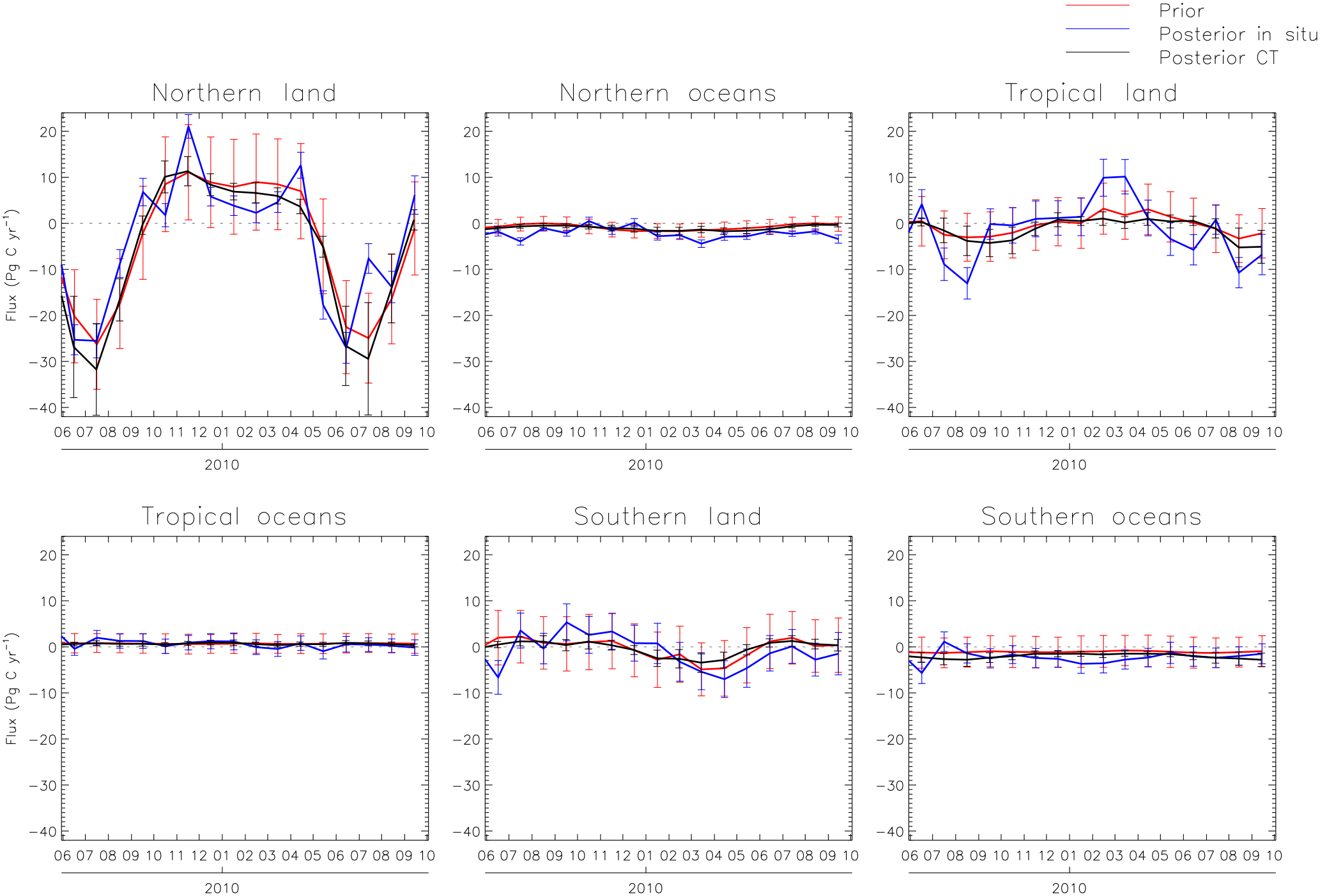
Figure 7Comparison of our in situ only inversion monthly mean NEP (× −1) and ocean fluxes, aggregated over large regions (as defined in TC3), with posterior fluxes from NOAA's CarbonTracker (CT2013B) data assimilation system. The priors shown are from our analysis; CT2013B priors are similar. Error bars represent 1σ uncertainties.

Download

Results from our in situ only inversion are shown alongside those of NOAA's CarbonTracker version 2013B inversion system (CT2013B) in Fig. 7 aggregated over large regions. CT2013B is an ensemble Kalman smoother data assimilation system with a window length of 5 weeks that uses multiple in situ observation networks and prior models to optimize weekly fluxes over 126 land “ecoregions” and 30 ocean regions (Peters et al., 2007; https://www.esrl.noaa.gov/gmd/ccgg/carbontracker/CT2013 B/CT2013B_doc.php, last access: 4 October 2016). Similar to the present study, CT2013B uses CASA-GFED3 fluxes from van der Werf et al. (2010) as one of the land NEP priors, though with different FPAR and meteorological driver data. (CASA-GFED2 is the other land prior in its ensemble of priors.) In addition, CT2013B uses the seawater pCO₂ distribution from the Takahashi et al. (2009) climatology to compute fluxes for one of its ocean priors; the other ocean prior is based on results from an atmosphere–ocean inversion. CT2013B uses a similar number of observation time series to that in the present study, 93 vs. 87. In Fig. 7, the two sets of posterior flux time series are similar overall, with overlapping 2σ ranges at all times except in the extratropical northern oceans region. One distinctive feature is that the posterior fluxes stay closer to the priors for CT2013B. A likely explanation is the tighter prior uncertainties in CT2013B, the magnitudes of which are on average 40 % of ours for land regions and 30 % of ours for ocean regions. For its ocean prior based on an atmosphere–ocean inversion, CT2013B assumes uncertainties consistent with the formal posterior uncertainties from the inversion, which are relatively small because of the large number of ocean observations used in the inversion; uniform fractional uncertainties are assumed for the other ocean prior and the land priors. Another feature is the larger month-to-month fluctuations in our results. In addition to the tighter prior uncertainties used, another factor that could contribute to smaller fluctuations in the CT2013B results is the use of prior estimates that represent a smoothing over three assimilation time steps, which attenuates variations in the forecast of the flux parameters in time. And another factor is that to dampen spurious noise due to the approximation of the covariance matrix by a limited ensemble, CT2013B applies localization for observation sites outside of the marine boundary layer, in which flux parameters that have a non-significant relationship with a particular observation are excluded. We further evaluate our inversions in the following sections.

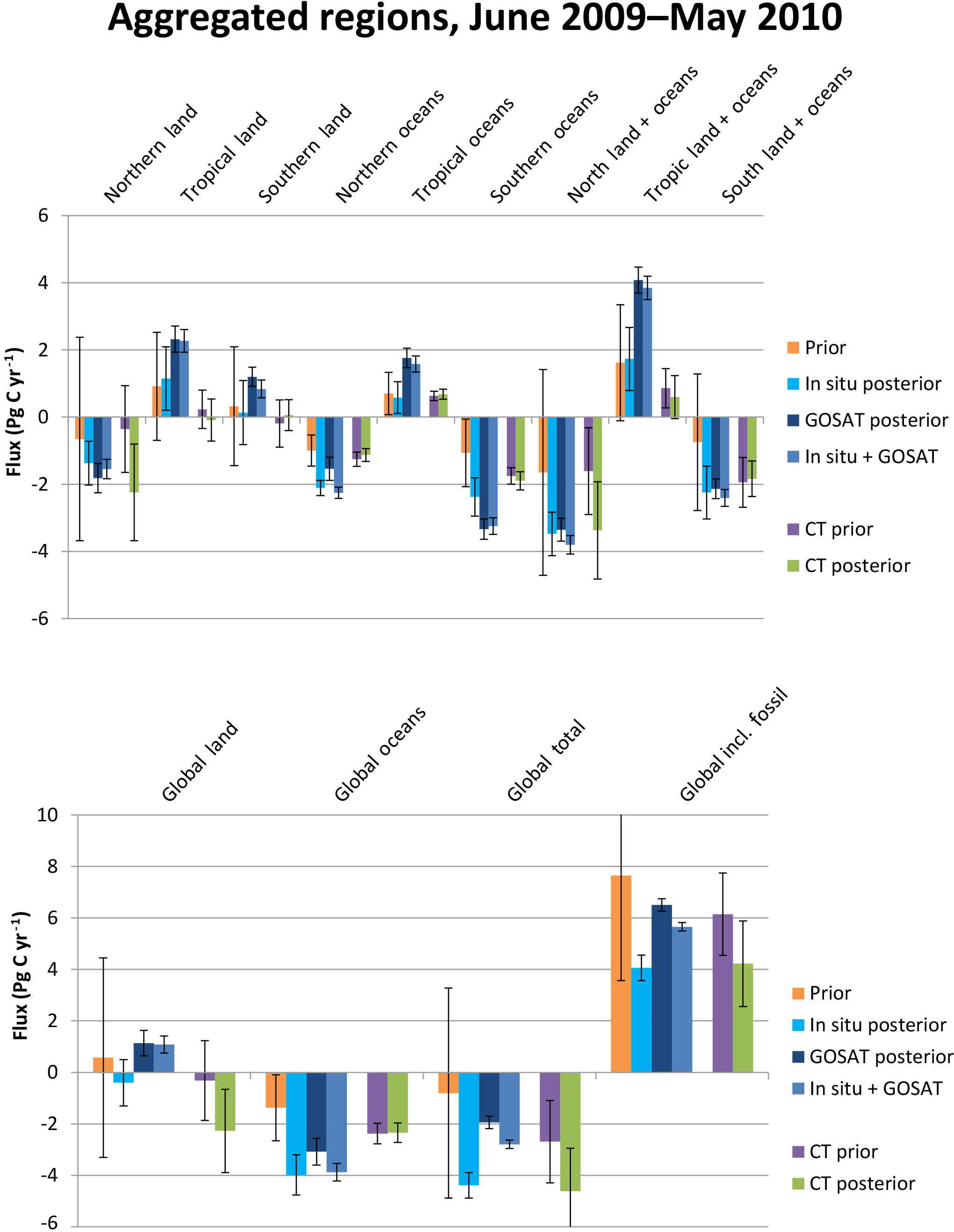
Figure 8Twelve-month mean NEP (× −1), fire, and ocean fluxes aggregated over large regions. Included are results for the in situ only, GOSAT only, and in situ + GOSAT inversions as well as priors. Shown for comparison are priors and posteriors from CT2013B. Error bars represent 1σ uncertainties; for CT2013B, “external” (across a set of priors) as well as “internal” (within a particular inversion) uncertainties are included. In summing monthly CT2013B fluxes over the 12 months, we assumed zero error correlation between months.

Download

3.2 Longer-term budgets and observation biases

Longer-timescale budgets can be assessed in Fig. 8, which displays 12-month mean fluxes (June 2009–May 2010) over large, aggregated regions, with fires now included, for our inversions and the CT2013B inversion. Results for individual TC3 regions are shown in Table 1. The global total flux (including fossil emissions) is substantially more positive for the GOSAT only inversion relative to the in situ only inversion, 6.5 ± 0.2 vs. 4.1 ± 0.5 Pg C yr⁻¹, while that for the in situ + GOSAT inversion lies in between at 5.7 ± 0.2 Pg C yr⁻¹. Such a large difference in the atmospheric CO₂ growth rate implied by the two distinct data sets is plausible even if there are no trends in uncorrected biases between the data sets, given their sampling of different regions of the atmosphere (e.g., total column vs. surface only) and the relatively short 12-month time frame over which the growth occurs. (In addition, the GOSAT data may be affected by modest trends and interannual variability in biases, as reported by Kulawik et al., 2016.) In fact, for a different 12-month period within our analysis, September 2009–August 2010, the total fluxes for the GOSAT only and in situ only inversions are much closer to each other – 5.53 and 5.47 Pg C yr⁻¹. Houweling et al. (2015) also found a larger total flux in the GOSAT only inversions relative to the in situ during June 2009–May 2010 averaged across eight models, ∼ 4.8 vs. ∼ 4.6 Pg C yr⁻¹, with a substantial amount of inter-model variability within those averages.

The GOSAT only inversion exhibits a shift in the global CO₂ sink from tropical and southern land to northern land relative to the prior and the in situ only inversion (Fig. 8). The differences are within the 1σ uncertainty ranges. The shift includes notable increases in the source in N. Africa, Temperate S. America, and Australia, and notable increases in the sink in Europe and Temperate N. America (Table 1). As for the ocean, the GOSAT inversion also exhibits a larger source in the tropics relative to the prior and the in situ inversion (outside of the 1σ ranges; Fig. 8). However, the GOSAT inversion now exhibits a smaller sink over extratropical northern oceans relative to the in situ inversion, and a larger sink over extratropical southern oceans relative to both the prior and the in situ inversion (at or outside of the 1σ ranges). The TC3 regions contributing the most to these differences include Tropical Indian, N. Pacific, N. Atlantic, and Southern Ocean (Table 1).

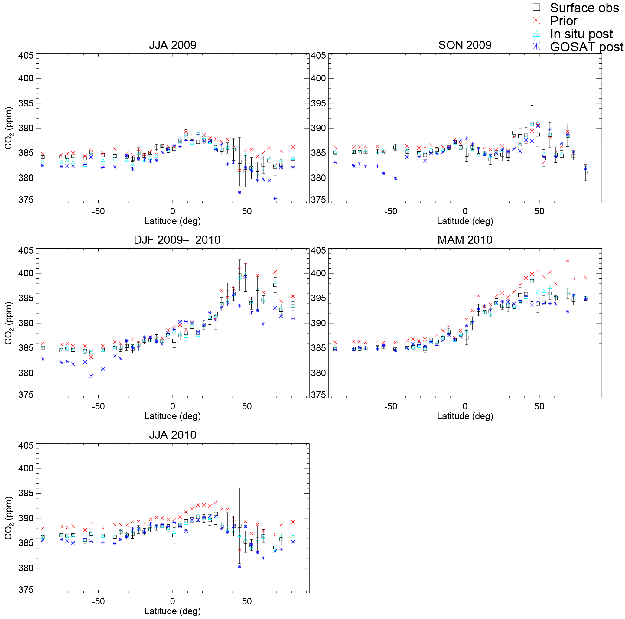
Figure 9Latitudinal profiles of seasonal mean CO₂ mole fractions at surface sites for observations, prior, in situ only posterior, and GOSAT only posterior. Values are averaged in 4^∘ bins. Error bars account for the spread in the observations within each season and bin as well as the uncertainty in each observation.

Download

The GOSAT results appear to contradict global carbon cycle studies that favor a weaker terrestrial net source in the tropics compensated by a weaker northern extratropical sink (e.g., Stephens et al., 2007; Schimel et al., 2015). We show the north–south land carbon flux partitioning of our results in Fig. S2 in the manner of Schimel et al. (2015). The shift in the sink from the south + tropics to the north in the GOSAT inversion relative to the in situ inversion goes in a direction opposite to that consistent with an airborne constraint considered by Stephens et al. (2007) and with the expected effect of CO₂ fertilization according to Schimel et al. (2015). However, the shift may be due at least in part to GOSAT retrieval and sampling biases. An evaluation of posterior mole fractions in the GOSAT only inversion against surface in situ observations indicates that the GOSAT inversion may be biased low during much of the analysis period over Europe and Temperate N. America, especially in winter (when there is little direct constraint at high latitudes by GOSAT observations), and biased somewhat high over N. Africa, especially in spring. However, the dearth of in situ sites over N. Africa, with only one in the middle of the region (in Algeria) and a few around the edges (e.g., Canary Islands and Kenya), precludes a definitive evaluation over that region. Globally, the GOSAT inversion tends to underestimate mole fractions at high latitudes of the Northern Hemisphere, often by more than 1σ, as shown by latitudinal profiles averaged over all surface sites by season (Fig. 9), suggesting an overestimated northern sink. The same is true of the high latitudes of the Southern Hemisphere. The GOSAT inversion overestimates mole fractions in parts of the tropics, sometimes by more than 1σ (Fig. 9), suggesting an overestimated tropical source. Uncorrected retrieval biases may be especially prevalent in the tropics, where there are very few TCCON stations available as input to the GOSAT bias correction formulas; only one TCCON station, Darwin, Australia, was operating in the tropics during 2009–2010, and only two more stations, Réunion (Reunion Island) and Ascension Island, became operational during the rest of the ACOS B3.4 retrieval period. In contrast, the posterior mole fractions for the in situ only inversion generally agree well with the surface observations (Fig. 9; also seen in the individual site time series in Fig. 2), which is expected given that these are the observations that are used in the optimization. The prior mole fractions are generally too high, which is consistent with the fact that the CASA-GFED biosphere is near neutral while the actual terrestrial biosphere is thought to generally be a net CO₂ sink.

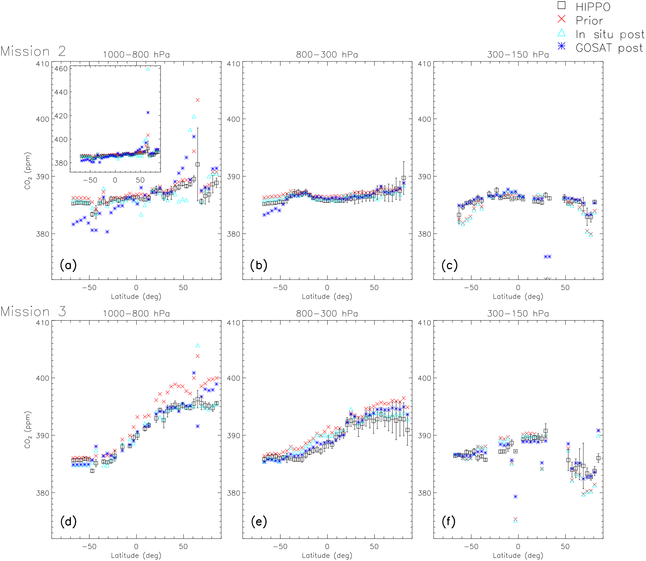
Figure 10Latitudinal profiles of CO₂ mole fractions for HIPPO observations and co-sampled prior, in situ only posterior, and GOSAT only posterior. Mission 2 (a–c) took place during 31 October–22 November 2009; Mission 3 (d–f) took place 24 March–16 April 2010. Values are averaged in three altitude bins and 4^∘ latitude bins. The inset in (a) contains an expanded y-axis range that shows two points that do not fit into the default range. Flight segments over the temperate North American continent (east of −130^∘) are excluded from this comparison in order to focus on the Pacific. Error bars represent the standard deviations of the observations within each bin.

Download

Evaluation of the inversions against latitudinal profiles constructed from HIPPO aircraft measurements, which provide additional sampling over the Pacific (Fig. 10), does not indicate any widespread overestimate by the GOSAT inversion relative to the observations in the tropics, unlike what was seen in Fig. 9 for comparison with the more globally distributed surface observations. But the GOSAT inversion does exhibit an underestimate relative to HIPPO from ∼ 40^∘ S southward in the lower to middle levels of the troposphere (Fig. 10a, b, d, e), especially for Mission 2 (October–November 2009). Again, retrieval bias and sampling bias (a lack of GOSAT ocean observations south of ∼ 40^∘ S and land observations south of ∼ 50^∘ S) are likely the causes of the underestimate. In the northern extratropics, the GOSAT inversion actually exhibits higher mean mixing ratios than HIPPO in general in the lower troposphere, especially for Mission 2, and the in situ inversion gives higher mixing ratios than HIPPO at some latitudes and lower mixing ratios at others for Mission 2. In one particular latitude range, 55–67^∘ N, both inversions give much higher mixing ratios than HIPPO, by up to 67 ppm in the case of the in situ inversion and 30 ppm for the GOSAT inversion. This could reflect inaccuracy in posterior fluxes due to the inversions being under-constrained over the high-latitude North Pacific and Alaska, with few observations during this season in the case of GOSAT and a tendency for the sparse in situ network to produce noisy inversion results, as was discussed above. However, given that the prior model also gives substantially higher mixing ratios than HIPPO at these latitudes (by up to 11 ppm), the discrepancy could be due in part to some factor common to the prior and posteriors such as model transport or representation error.

In the upper troposphere to lower stratosphere, the GOSAT inversion more often than not exhibits better agreement with the HIPPO observations than the in situ inversion does for both Mission 2 and Mission 3 (Fig. 10c, f). (We think it is reasonable to include data from these altitudes as part of the evaluation of the inversion results, since the tropopause in the GEOS-5/MERRA meteorological data assimilation system underlying PCTM transport is considered to be accurate; Wargan et al., 2015; and PCTM has been shown to simulate upper troposphere-lower stratosphere trace gas gradients well compared to other models; Patra et al., 2011.) This may have to do with the fact that the GOSAT data provide constraints throughout the atmospheric column, whereas the in situ measurements constrain only surface CO₂. Given the lack of high-altitude constraints, the in situ inversion should not be expected to improve agreement with high-altitude aircraft observations relative to the prior, and, indeed, the inversion is no better than the prior (Fig. 10c, f). Note that the GOSAT data may not be driving the mole fraction adjustments locally in the region evaluated here, given the relative sparseness of GOSAT retrievals over the ocean, especially at high latitudes during the times of year of the HIPPO missions. Rather, the GOSAT data set provides large-scale atmospheric constraints that are transmitted to this region by transport. A possible explanation for the better agreement of the GOSAT inversion with HIPPO observations at these higher altitudes than at lower altitudes is that air parcels at higher altitudes generally consist of mixtures of air originating from broader areas near the surface (e.g., Orbe et al., 2013), so that regional posterior flux errors are more likely to cancel out (e.g., due to combining of negatively correlated errors from different regions), especially in the upper troposphere or above.

The conclusion that GOSAT biases may contribute to the shift in the land sink is also supported by Houweling et al. (2015). That study reported a shift in the GOSAT only inversions relative to the in situ inversions consisting of an increase in the sink in northern extratropical land of 1.0 Pg C yr⁻¹ averaged across models and an increase in the source in tropical land of 1.2 Pg C yr⁻¹ during June 2009–May 2010; in comparison, our inversions produce an increase in the northern land sink of 0.4 Pg C yr⁻¹ and an increase in the tropical land source of 1.2 Pg C yr⁻¹ (Fig. 8). Houweling et al. (2015) found an especially large and systematic shift in flux of ∼ 0.8 Pg C yr⁻¹ between N. Africa and Europe, but then provided evidence that the associated latitudinal gradient in CO₂ mole fractions may be inconsistent with that based on surface and HIPPO aircraft in situ observations. They also suggested that the shift in annual flux between the two regions may be a consequence of sampling bias, with a lack of GOSAT observations at high latitudes during winter. Chevallier et al. (2014) also found a large source in N. Africa of ∼ 1 Pg C yr⁻¹ in their ensemble of GOSAT inversions and considered the magnitude of that unrealistic, given that emissions from fires in that region likely amount to < 0.7 Pg C yr⁻¹. (Note that our N. Africa source is even larger than that of Chevallier et al., 2014.) Inversion experiments by Feng et al. (2016) provide evidence that the large European sink inferred from GOSAT observations may be an artifact of high XCO₂ biases outside of the region that necessitate extra removal of CO₂ from incoming air for mass balance, in concert with sub-ppm low XCO₂ biases inside the region. An observing system simulation experiment by Liu et al. (2014) found that GOSAT seasonal and diurnal sampling biases alone could result in an overestimated annual sink in northern high-latitude land regions. And a review paper by Reuter et al. (2017) further highlighted the discrepancy between satellite-based and ground-based estimates of European CO₂ uptake and cited retrieval and sampling biases as possible sources of error in the former (while also noting sampling issues with in situ networks for the region).

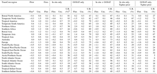
Again, the results for the in situ + GOSAT inversion lie mostly in between those for the in situ only and GOSAT only inversions, with the in situ + GOSAT fluxes lying closer to the GOSAT only ones for the tropical and southern land regions and land as a whole (Table 1 and Fig. 8), suggesting the dominance of the GOSAT constraint in these regions. The posterior uncertainties for the GOSAT inversion (Table 1) are as small as or smaller than those for the in situ inversion, except in Boreal and Temperate N. America, N. Pacific, Arctic/Northern Ocean', and Southern Ocean. This reflects the fact that GOSAT generally provides better spatial coverage, except over N. America, where the in situ network provides good coverage, and over and near high-latitude ocean areas, where there is fairly good in situ coverage and poor GOSAT coverage. Uncertainty reductions in the in situ inversion range from 15 to 93 % for land regions and 15 to 56 % for ocean regions (Table 1). In the GOSAT inversion, the uncertainty reductions range from 43 to 89 % for land and 19 to 56 % for ocean. And in the inversion with combined in situ and GOSAT data, the uncertainty reductions are larger than or equal to those in either the in situ only or the GOSAT only inversion, ranging from 61 to 96 % for land and 40 to 67 % for ocean.

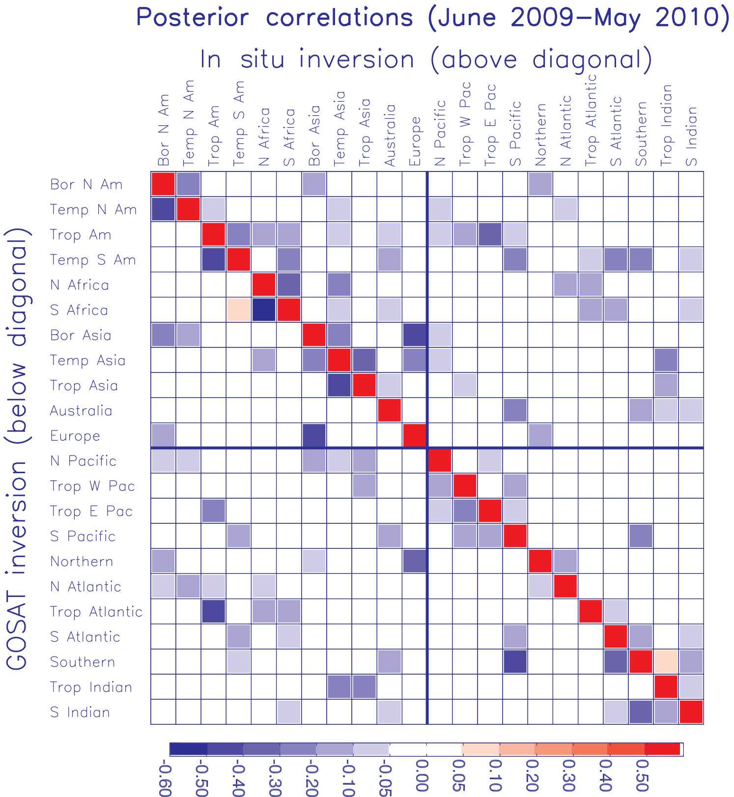
Figure 11Posterior spatial flux error correlations, aggregated to TC3 regions and a 12-month period, for the in situ only inversion (for compactness, shown on and above the main diagonal), and the GOSAT only inversion (on and below the diagonal). The correlation is equal to the error covariance divided by the product of the corresponding flux uncertainties (σ). Values on the diagonal are equal to 1.

Download

3.3 Flux error correlations and land–ocean partitioning

Here we elaborate on posterior error correlations, which indicate the degree to which fluxes are estimated independently of one another. Negative correlations can be manifested in dipole behavior, in which unusually large flux adjustments of opposite signs occur in neighboring regions/time intervals. Spatial error correlations are shown in Fig. 11 aggregated to TC3 regions and the 12-month period from June 2009 to May 2010. The full-rank error covariance matrix generated by the exact Bayesian inversion method (from which the correlation coefficients are derived) is a unique product of this study, particularly as applied to satellite data. There are a larger number of sizable correlations between land regions in the in situ inversion than in the GOSAT inversion (in the top left quadrant of the plot). One specific feature is negative correlations among the four TC3 regions in South America and Africa (“Trop Am”, “Temp S Am”, “N Africa”, and “S Africa”) in the in situ inversion, whereas in the GOSAT inversion there are negative correlations within South America and within Africa but not between the two continents. Although there are less extensive correlations over land in the GOSAT inversion, they are often of larger magnitude than in the in situ inversion; this could reflect the fact that GOSAT observations, though of higher density than the in situ observations over many regions, are column averages representing mixtures of air from a broader source region than for surface observations, and may thus result in larger error correlations for immediately adjacent regions, e.g., within a continent. Over the ocean regions, in contrast, the GOSAT inversion exhibits anti-correlations that are as extensive as those for the in situ inversion and often of larger magnitude. For example, there are substantial negative correlations between Southern Ocean and each of the other southern regions – S. Pacific, S. Atlantic, and S. Indian. This is consistent with the almost complete lack of GOSAT observations at the latitudes of the Southern Ocean region and the southern edges of the neighboring ocean regions (Fig. 1b). Interestingly, there is not a sizable correlation between N. Africa and Europe in the GOSAT inversion (in either seasonal or 12-month means), which runs counter to what might be expected from the shift in flux discussed above; rather, each of these regions is correlated with a number of other regions. We do find a fairly large correlation of −0.62 between the northern extratropics in aggregate (land + ocean) and the tropics for the 12-month period though. Correlations for the in situ + GOSAT inversion (not shown) generally lie in between those of the in situ only and GOSAT only inversions. Even with the incorporation of both sets of observations, there are substantial correlations of as much as −0.6 between regions within a continent, reinforcing our earlier conclusion that sampling gaps limit the ability of the observations to constrain fluxes down to the scale of most TC3 regions.

The in situ only and CT2013B posterior global totals are nearly the same, but the land–ocean split is different, with our inversion exhibiting a larger sink over ocean than over land (with non-overlapping 2σ ranges) while in CT2013B the land and ocean fluxes are similar, with the ocean flux changing little from the prior (Fig. 8). A likely explanation for the difference is the very tight prior constraints on ocean fluxes of CT2013B that were discussed above, which force the flux adjustments to take place mostly on land. The GOSAT inversion also exhibits a relatively large ocean sink of −3.1 ± 0.5 Pg C yr⁻¹; for comparison, the CT2013B estimate is −2.4 ± 0.4 Pg C yr⁻¹, our in situ only estimate is −4.0 ± 0.8 Pg C yr⁻¹, and the estimate of the Global Carbon Project (GCP) is −2.5 ± 0.5 Pg C yr⁻¹ for 2009–2010 (Le Quéré et al., 2013, 2015). The GCP estimate is a synthesis that combines indirect observation-based estimates for the mean over the 1990s with interannual variability from a set of ocean models and accounts for additional observation-based estimates in the uncertainty. The difference between our inversion estimates and the GCP estimate is actually even larger than suggested by those numbers, given that a background river to ocean flux of ∼ 0.5 Pg C yr⁻¹ should be subtracted from our ocean flux to make it comparable to the GCP ocean sink, which refers to net uptake of anthropogenic CO₂ (Le Quéré et al., 2015). Our relatively small land sink is reflected in our inversion results lying mostly outside of the GCP global land flux range in the north–south partitioning plot in Fig. S2. Similarly, in comparing our results with those of Houweling et al. (2015), we find that the global budgets are comparable for all three inversions – in situ only, GOSAT only, and in situ + GOSAT – as was mentioned above, but the land–ocean split is different. Our posterior ocean flux is −4.0 ± 0.8, −3.1 ± 0.5, and −3.9 ± 0.3 Pg C yr⁻¹ for the three inversions, while it is −1.6 ± 0.5, −1.2 ± 0.6, and −1.5 ± 0.8 Pg C yr⁻¹ in the results of Houweling et al. (2015; Sander Houweling, personal communication, 2016) (averaged over different weighted averages of the models).

There is a strong negative correlation globally between posterior flux errors for land and ocean of −0.84 and −0.89 in the in situ only and the GOSAT only inversion, respectively. Basu et al. (2013) also reported a large negative correlation between land and ocean fluxes of −0.97 in their in situ + GOSAT inversion during September 2009–August 2010. The anti-correlations imply that the observations cannot adequately distinguish between adjustments in the global land and ocean sinks. Thus, land–ocean error correlation may be a fundamental challenge that global CO₂ flux inversions are faced with, at least given the sampling characteristics of the in situ and GOSAT data sets used here. Without tight prior constraints on ocean fluxes, those fluxes are subject to large, and potentially unrealistic, adjustments (i.e., dipole behavior).

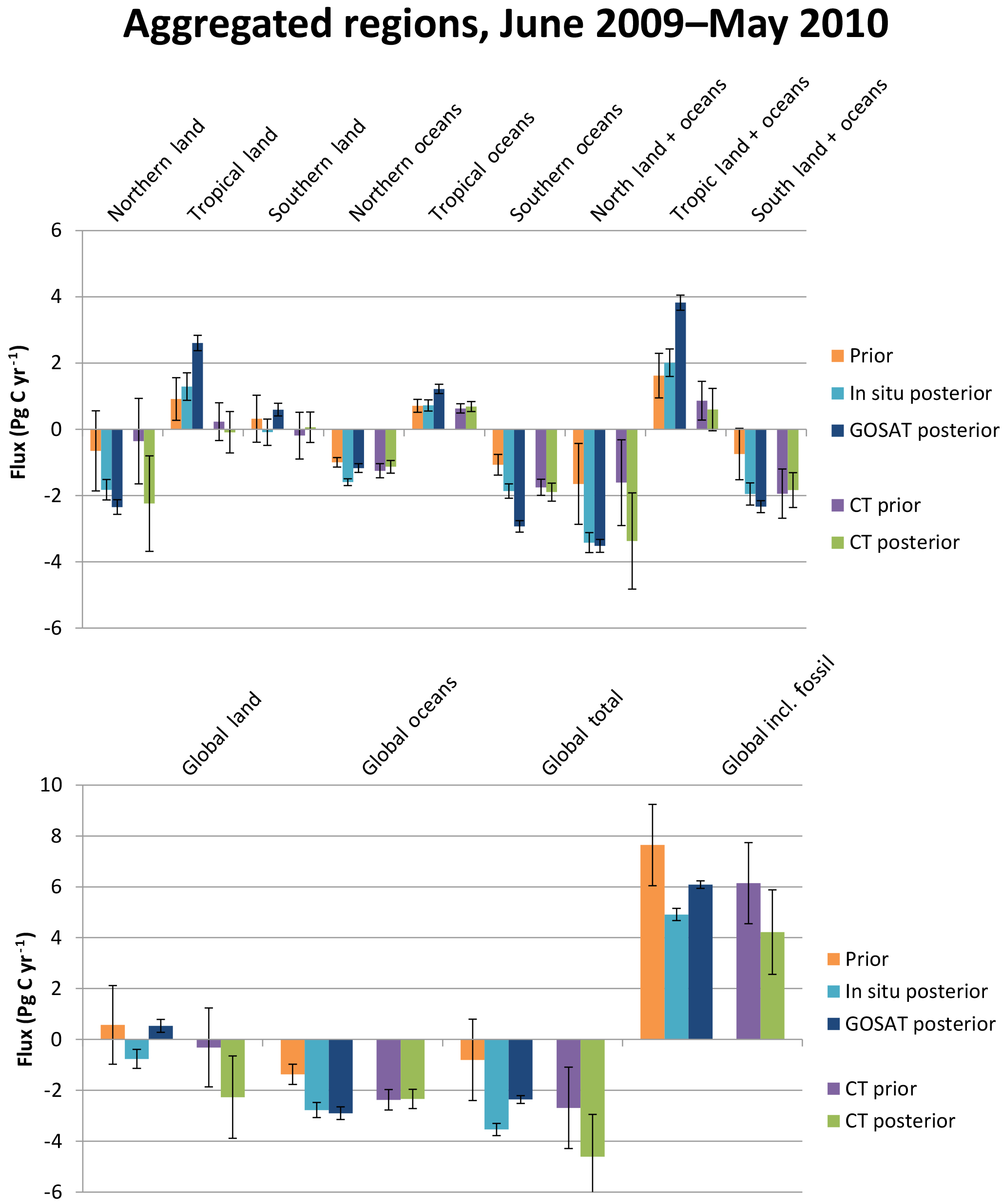
Figure 12Similar to Fig. 8, except showing results for inversions with tighter prior constraints (with prior uncertainties similar to CarbonTracker's). Included are results for the in situ only and GOSAT only inversions. CT2013B results shown in Fig. 8 are repeated here. Error bars represent 1σ uncertainties.

Download

To assess the effect of prior constraints on the inversion, we conducted a test with reduced prior uncertainties, for both land and ocean fluxes, so that they are similar on average to those of CT2013B. Results for an in situ only inversion and a GOSAT only inversion are shown in Table 1 and Fig. 12. For the in situ only inversion, the posterior ocean flux is now much smaller in magnitude, −2.8 ± 0.3 Pg C yr⁻¹. The posterior ocean flux for the GOSAT inversion does not change as much, decreasing in magnitude from the original −3.1 ± 0.5 to −2.9 ± 0.2 Pg C yr⁻¹. The ocean flux 1σ ranges for both inversions now overlap with the 1σ range of CT2013B; accounting for the riverine flux, the 1σ range for the in situ inversion overlaps with the 1σ range of GCP, while the 1σ range for the GOSAT inversion is still just outside that of GCP. The better agreement with the GCP budget (land component) can also be seen in Fig. S2 for both inversions. The inversions with tighter priors have slightly larger cost function values than the baseline inversions (Table 2; the difference for the GOSAT cases is concealed by rounding). The inversions with tighter priors generally exhibit slightly better agreement with independent observations, e.g., lower-altitude HIPPO observations (Fig. S3), and surface observations in the case of the GOSAT inversion (Fig. S4), indicating that the effects of sampling and retrieval biases are reduced with tighter prior uncertainties. The better agreement also lends support to the smaller ocean sink estimates. (At high altitudes, keeping posterior mole fractions closer to the prior mole fractions results in worse agreement with HIPPO in many places, especially for the GOSAT inversion.) However, the tighter priors do not completely eliminate the discrepancies between the inversions and the independent observations, suggesting that tight priors may not completely counteract the effects of observational biases.

Basu et al. (2013) saw a similar underestimate of mole fractions during parts of the year in the southern extratropics in their GOSAT inversion relative to surface observations and overestimate of the seasonal cycle, though with some differences in the shape of the seasonal cycle from our study (including a later descent toward and recovery from the annual minimum in austral summer and a larger peak in late winter-early spring). They, however, used the SRON-KIT RemoTeC GOSAT retrieval with a known issue over the ocean, and concluded that adding global land and ocean observation bias correction terms to their inversion was needed to make the land–ocean flux split more realistic and to improve the seasonal cycle of CO₂ in the southern extratropics. In contrast, studies have found no noticeable bias in the ACOS B3.5 ocean glint XCO₂ retrievals relative to TCCON (Kulawik et al., 2016) and a mean bias of only −0.06 ppm relative to HIPPO (Frankenberg et al., 2016); the B3.4 version we use is on average ∼ 0.2 ppm lower than B3.5 in 2010 (Deng et al., 2016). So although a small overall negative bias in the bias-corrected ACOS B3.4 ocean data cannot be ruled out (and there could of course be larger negative biases on a regional scale, such as in the southern extratropics), we conclude that the land–ocean flux split in inversions using either in situ or GOSAT data is strongly influenced by error correlations and dependent on the prior uncertainties assumed.

The shift in the global terrestrial sink from the tropics and south to the north when comparing the GOSAT only inversion with the in situ only inversion and the prior is still seen when prior uncertainties are decreased (Figs. 12, S2), as is a substantially more positive global total budget in the GOSAT inversion relative to the in situ (Fig. 12). The uncertainty reductions in the test inversions are smaller than those in the baseline inversions (Table 1), as is expected from the smaller starting values of the uncertainties. In summary, the magnitude of the ocean sink and the partitioning of the global sink between land and ocean are sensitive to the prior uncertainties, but other inferred features of the carbon budget are robust with respect to prior uncertainties.

Given that there is uncertainty in the land–ocean flux partitioning at sub-global scales as well (e.g., as indicated by moderate negative correlations between northern land and northern oceans, tropical land and tropical oceans, etc.), we consider results for combined land and ocean regions in Figs. 8 and 12. They indicate that there is a shift in the global sink from the tropics to the north and the south in the GOSAT inversion relative to the prior, and an increased source in the tropics of ∼ 2 Pg C yr⁻¹ in the GOSAT inversion relative to the in situ inversion. These features are seen in the inversions with tighter priors as well as in the baseline inversions. Note that the increased source over southern land and increased sink over southern oceans in the GOSAT inversion relative to the in situ inversion that were discussed earlier cancel each other out approximately, suggesting a compensation of errors. Also note that the inversion using the in situ + GOSAT data sets, which provide more constraint than either of the data sets alone, produces a global flux close to midway between the in situ only and GOSAT only inversions, while it produces a Tropic Land + Oceans flux much closer to that of the GOSAT inversion than to the in situ inversion. This suggests some degree of independence of the GOSAT-inferred regional result from the global result.

3.4 Impacts of climatic conditions on 2009–2010 fluxes

We now analyze the impacts of several climatic events during the analysis period on CO₂ fluxes as indicated by the inversion results. We focus on (1) unusually hot and dry conditions at Northern Hemisphere, higher latitudes in summer of 2010, (2) wetter conditions over parts of North America in spring and early summer of 2010 relative to 2009, and (3) record drought in the Amazon in 2010.

Guerlet et al. (2013), who examined GOSAT data and performed a flux inversion using a variational assimilation system, found that there was less net terrestrial CO₂ uptake in summer of 2010 than in 2009 at northern high latitudes, consistent with known severe heat waves, drought, and high fire emissions, especially across Eurasia, centered around western Russia, and to a lesser extent in North America.

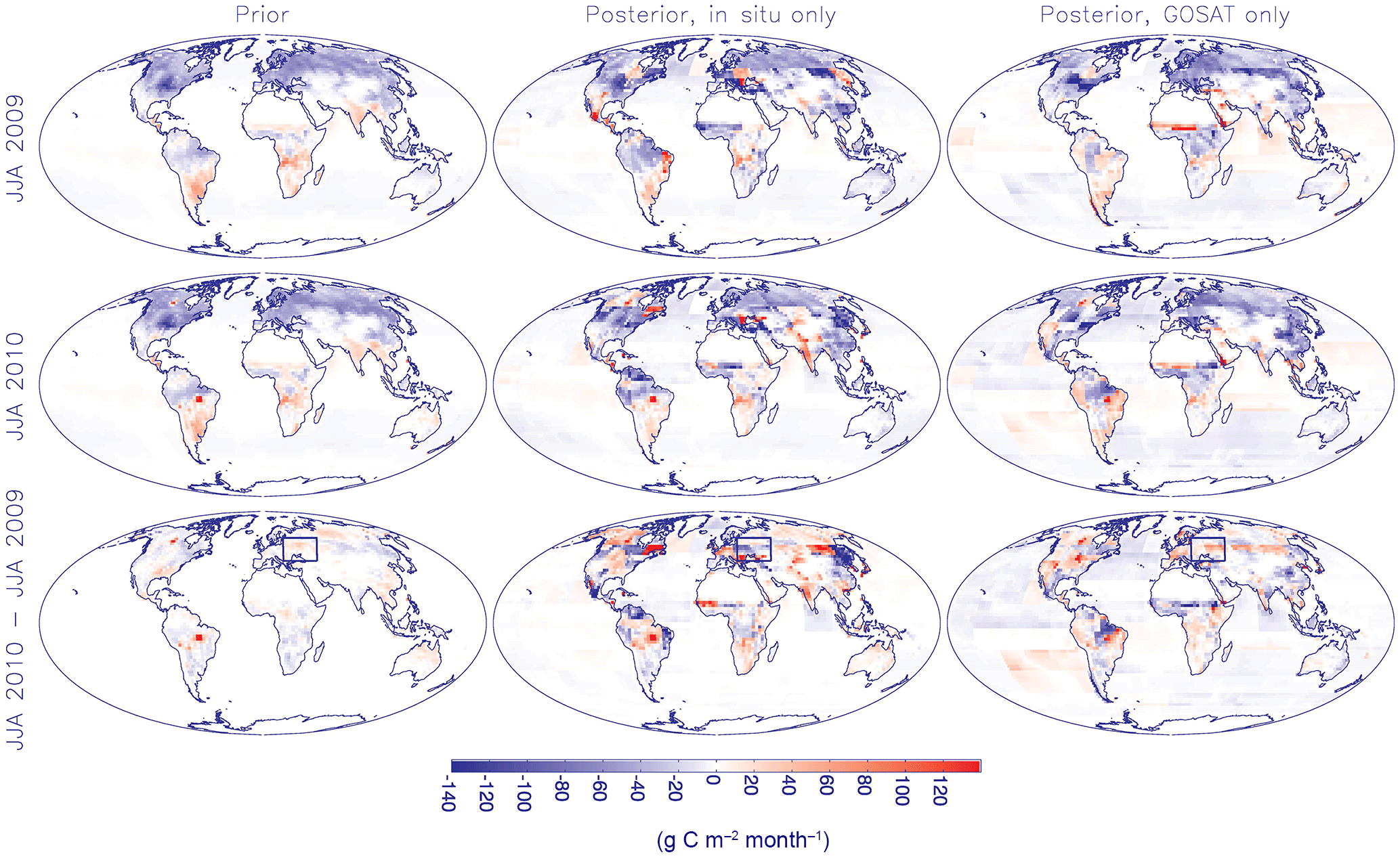
Figure 13Comparison of spatial distribution of fluxes for June–July–August of 2010 vs. 2009. Included are natural and fire fluxes. Shown are fluxes for 2009 (top), 2010 (middle), and the 2010–2009 difference (bottom), for the priors (left), in situ only inversion (middle), and GOSAT only inversion (right). In the bottom row, boxes enclose the region around western Russia where there were intense heat waves, severe drought, and extensive fires. Note that the grid-scale spatial variability shown is not optimized in the inversions, so only patterns at the scale of the 108 flux regions contain information from the observations.

Download

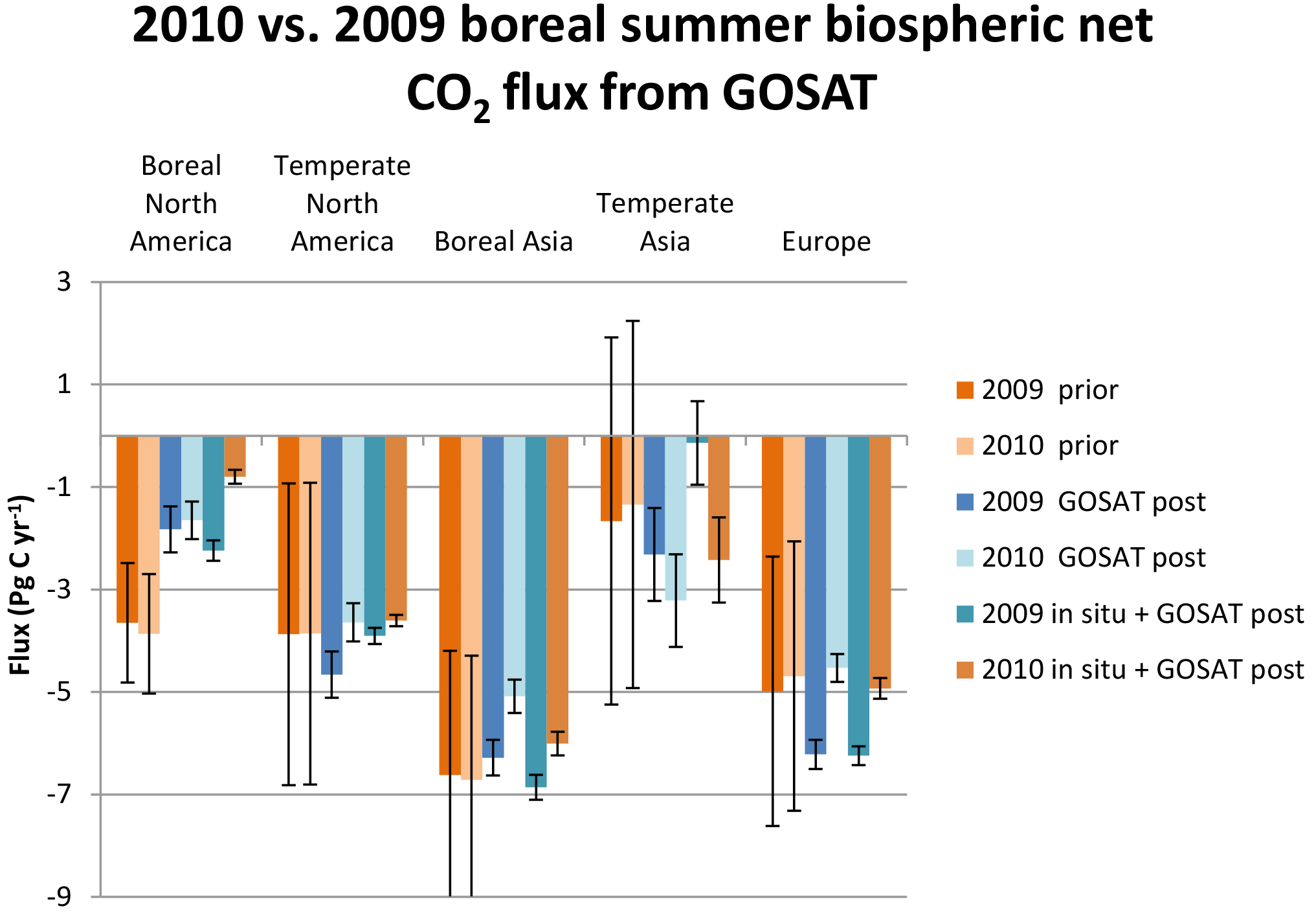
Figure 14Comparison of prior, GOSAT only posterior, and in situ + GOSAT posterior fluxes aggregated over northern regions for June–July–August of 2010 vs. 2009. Included are NEP (× −1) and fire fluxes. Error bars represent 1σ uncertainties.

Download

Motivated by that study, we examined our inversion results for 2009 and 2010, focusing on the GOSAT inversion. As can be seen in the global maps of natural plus biomass burning fluxes in June–July–August (JJA) in Fig. 13, the GOSAT inversion does appear to exhibit a decreased CO₂ uptake over Eurasia, including the area around western Russia (enclosed in a box in the figure), in 2010. A decreased sink can also be seen in parts of North America. A decreased sink over western Russia can also be seen in the CASA-GFED prior, though of a smaller magnitude. In contrast, there is actually an increased sink in that region in the in situ inversion. In fact, none of the sites used are in or immediately downwind of that region (Fig. 1a). Total NEP and fire fluxes over northern TC3 regions are shown in Fig. 14. There is less CO₂ uptake in JJA 2010 than in 2009 in all the regions except Temperate Asia in the GOSAT only inversion. The differences exceed the 1σ ranges for three of the five regions, even exceeding the 3σ ranges for Europe, which includes western Russia. Also shown is the in situ + GOSAT inversion, which exhibits a similar pattern of 2010–2009 differences. These inversion results are thus consistent with the earlier GOSAT study. In contrast, the 2010–2009 differences in the prior are small and, for some regions, of the opposite sign as that in the inversions (Fig. 14).

Table 3Mean 2010–2009 difference in mole fractions over June–July–August at Siberian sites (in ppm).

Download Print Version | Download XLSX

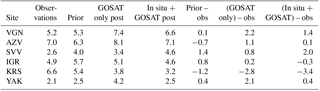
Measurements from the JR-STATION tower network are suitably located for evaluating the inferred flux interannual variability over Eurasia. Time series are shown in Fig. 15 for observations, the prior model, and the GOSAT only inversion at six sites with complete summertime data in 2009–2010. (As with the continuous measurements used in the in situ inversion, afternoon data are selected to avoid difficulties associated with nighttime boundary layers.) Posterior mole fractions are noisier in the wintertime, likely a result of the lack of GOSAT observations during that season at these high latitudes. Focusing on 2010–2009 differences, the observations suggest a shallower drawdown in 2010 than in 2009 at most of the sites, which is generally captured by both the prior and the GOSAT posterior. It appears though that the GOSAT inversion exaggerates the 2010–2009 difference at some of the sites, overestimating especially the drawdown in 2009. For a more quantitative analysis, we calculate the average 2010–2009 difference in mole fractions over June–July–August for each site (Table 3). The GOSAT only inversion overestimates the 2010–2009 difference at five of the six sites. The in situ + GOSAT inversion exhibits less of an overestimate overall than the GOSAT only inversion, with three of the six sites being substantially overestimated. The prior exhibits the best agreement with the observations overall.

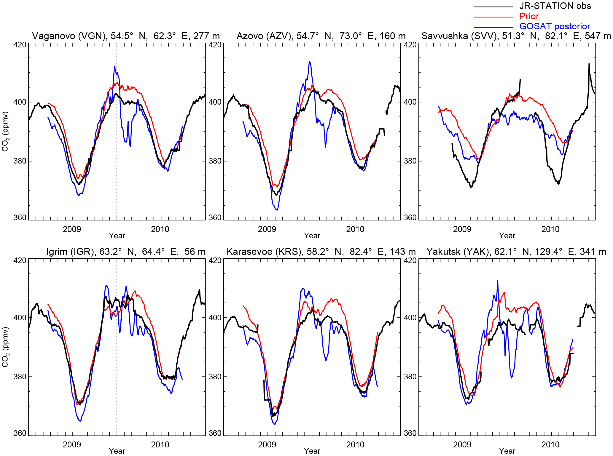
Figure 15Evaluation of the prior model and GOSAT only inversion against JR-STATION in situ observations in Siberia. Shown are daily afternoon average (12:00–17:00 LT, local time) mole fractions from the highest level on each tower, the time series of which are smoothed with a 31-day window. Sites are arranged from west to east, first at lower latitudes and then at higher latitudes, excluding those with data gaps in the summer. Elevations shown include intake heights on towers.

Download

The earlier study by Guerlet et al. (2013) assumed that the differences between 2010 and 2009 posterior biospheric fluxes are relatively insensitive to biases in the GOSAT data, since at least some of those errors may be similar between the two years. However, our evaluation of the inversions using JR-STATION data suggests that retrieval biases can vary significantly from year to year. Kulawik et al. (2016) estimated a year-to-year variability in GOSAT biases relative to TCCON of 0.3 ppm averaged over the stations. Another study has raised a separate but related issue of inversion results potentially being sensitive to the spatiotemporal distribution of observations in different data sets (e.g., different GOSAT retrievals) (Hiroshi Takagi, personal communication, 2015); by extension, comparison of fluxes from two time periods can be affected by changes in the distribution of observations over time within a particular data set. But in JJA 2009 and 2010, there are similar numbers of ACOS GOSAT observations overall in the northern land region, so differences in data coverage are probably not a factor in this particular case study.

Our evaluation using JR-STATION data also indicates that the prior may be a reasonable estimate of the 2010–2009 difference in growing season fluxes, at least over Siberia, despite possible shortcomings in the simulation of drought impacts on NEP and of the overall magnitude of fire emissions by CASA-GFED3. The latest version of GFED (version 4s), which includes small fires, tends to generate higher emissions than GFED3 (van der Werf et al., 2017).

Over large parts of North America, conditions were wetter in spring and early summer of 2010 than in 2009, especially in the western half of the US and adjacent parts of Mexico and Canada, as suggested by North American drought maps for June 2010 vs. June 2009 (e.g., https://www.drought.gov/nadm/content/map/2010/06, last access: 12 July 2016) and shallow groundwater status maps for the US based on GRACE (Gravity Recovery and Climate Experiment) satellite data for May–June (Houborg et al., 2012; http://nasagrace.unl.edu/Archive.aspx, last access: 19 July 2018). Consistent with the wetter conditions in 2010 are a larger CO₂ sink over North America (Boreal + Temperate) in May–June 2010 relative to 2009 in our priors (−5.0 ± 3.9 vs. −3.4 ± 3.9 Pg C yr⁻¹), in situ only posteriors (−5.0 ± 0.4 vs. −3.8 ± 0.5 Pg C yr⁻¹), and GOSAT only posteriors (−5.8 ± 0.4 vs. −3.3 ± 1.8 Pg C yr⁻¹). We consider the in situ inversion result to be reliable here, given the large uncertainty reduction for North America and small error correlations with other regions (not shown). The 2010 and 2009 fluxes differ such that their 1σ ranges do not overlap for the in situ and the GOSAT posteriors. Much warmer conditions in eastern North America in May–June 2010 compared to 2009 (e.g., https://www.ncdc.noaa.gov/sotc/global/201005, last access: 6 April 2018 and https://www.ncdc.noaa.gov/sotc/global/200905, last access: 6 April 2018) may have also contributed to increased uptake, especially at higher latitudes, where insufficient warmth can be more of a limiting factor for NEP than insufficient moisture during late spring to early summer. Despite the increased sink in June 2010 over North America, the 2010 summer exhibits a decreased sink relative to 2009 when integrated through June–July–August (Fig. 14).

The Amazon basin experienced a record drought in 2010, which led to decreased vegetation greenness and a net carbon loss to the atmosphere (Xu et al., 2011; Gatti et al., 2014). Dry conditions in the north and center of the basin in the first three months were caused by the El Niño of late 2009 to early 2010, and an enhanced and prolonged dry season in the southern areas of the basin was connected to an Atlantic sea surface temperature anomaly during the second half of the year (Gatti et al., 2014). According to our prior estimate, fire emissions minus NEP represented a near-zero net flux of −0.1 ± 2.1 Pg C yr⁻¹ in July–September 2010 (a period that includes peak drought conditions and fire counts of that year) and a sink of −1.9 ± 2.1 Pg C yr⁻¹ in July–September 2009 in the TC3 Tropical America region. (The fire emissions amounted to 2.0 and 0.2 Pg C yr⁻¹ in July–September 2010 and 2009, respectively, while NEP was 2.1 Pg C yr⁻¹ in both periods.) However, our GOSAT inversion suggests the reverse, −0.9 ± 0.6 vs. −0.4 ± 0.3 Pg C yr⁻¹ for July–September 2010 and 2009, respectively. (We do not report the analogous results for the in situ inversion, since the uncertainties are large in this undersampled region.) The prior estimate seems more consistent with the expected impact of drought on fluxes than the inversion estimate does. The inversion is hampered in the region by the relatively small number of GOSAT soundings that are retrieved and pass the quality filters, especially during the burning season (with substantial light scattering by aerosols) and the rainy season (with extensive cloud cover). The dearth of observations results in relatively large posterior uncertainties and/or sizable flux error correlations. Furthermore, there is differing data coverage, with 2010 having fewer observations than 2009 in the TC3 Tropical America region during the height of the fire season (85 and 20 in August and September 2010, respectively, vs. 101 and 33 in 2009) and more observations than 2009 in July (150 vs. 85). The differing data coverage itself could affect the flux estimates differently in 2009 and 2010. The Amazonica data set does not enable an evaluation of the flux estimates for both 2009 and 2010, since the data set begins in 2010. However, comparison of the prior and GOSAT model mole fractions in 2010 with the Amazonica data shows that biases for both can vary substantially over time, e.g., in July vs. August–September (Fig. S1). This raises the possibility that neither the prior nor the GOSAT inversion correctly estimates the interannual flux difference in this region and also supports the idea that inversion bias can vary with data coverage.