BUILD A TENSORFLOW OCR IN 15 MINUTES WITH DEEP LEARNING TECHNOLOGY
 Datamites Team

Hello and welcome to DATAMITES, home of data science.
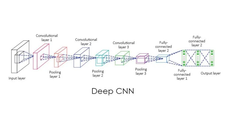
Hello everyone and welcome to the data convolutional neural network code along in this lecture. We’re going to connect the theory ideas that we previously talked about to actual implementation of code tensorflow. Let’s open up a Jupiter notebook and get started.
PROBLEM OVERVIEW
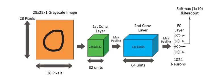
Here, the problem set we have is the MNIST dataset and what we are trying to achieve is to build an image recognition algorithm that can successfully classify the images in to any digit from 1 to 9.The MNIST dataset contains 57,000 train images and 5000 test images of handwritten characters from 0 to 9.
So the first thing I’m going to do is import Tensor flow of course as T.F. and then I’m going to set up the data just like we did before. This imports our input data then we’ll say this is equal to input data function and then we’re going to call read data sets on this function. And we’ll set one hot equal to true, to make sure that our output features [numbers from 1 to 9] are one hot encoded as a 10*10 matrix of features.
importtensorflow as tf
fromtensorflow.examples.tutorials.mnist import input_data
mnist = input_data.read_data_sets(“MNIST_data/”,one_hot=True)
CREATION OF HELPER FUNCTIONS:
Next,I’m first going to create a couple of helper functions I’m first going to create a
1.helper function that will help me initialize the weights Of a layer.
2.The next one is going to help initialize the bias of a layer.
3.then we’ll have some other ones that do return a 2D convolution. So basically taking a tensor and taking a filter and apply it as a convolution and then also do a pooling helper function.
definit_weights(shape):
init_random_dist = tf.truncated_normal(shape, stddev=0.1)
returntf.Variable(init_random_dist)
definit_bias(shape):
init_bias_vals = tf.constant(0.1, shape=shape)
returntf.Variable(init_bias_vals)
def conv2d(x, W):
return tf.nn.conv2d(x, W, strides=[1, 1, 1, 1], padding=’SAME’)
Remember our input tensor is going to be a bunch of images so that’s the batch dimension that we have the height and width of an individual image and then the color channel. So the only basically pooling that I want is along the height and width of an individual image which means as far as the size is concerned I’m going to have a two by two along the height and width. So that’s the actual pooling. And then a again along the channels and I’m going to do the same thing for stride. So we’re going to stride by two.
CREATION OF POOLING LAYER:
def max_pool_2by2(x):
returntf.nn.max_pool(x, ksize=[1, 2, 2, 1],
strides=[1, 2, 2, 1], padding=’SAME’)
CREATION OF CONVOLUTIONAL LAYER:
In this function in fact we’ll just call it a “convolutional layer” is going to take some input X and then the shape parameter so we’ll create the weights with the shape and the biases are just going to run along the third dimension. So I’ll say it biases and then we’re just going to pass in shape three here. And then I’m going to return T.F. tensor flow object. I’m going to use a rectified linear unit as the activation function.
Using the conv2d function, we’ll return an actual convolutional layer here that uses anReLu activation.
defconvolutional_layer(input_x, shape):
W = init_weights(shape)
b = init_bias([shape[3]])
returntf.nn.relu(conv2d(input_x, W) + b)
CREATION OF FULLY CONNECTED LAYER:
This is a normal fully connected layer
defnormal_full_layer(input_layer, size):
input_size = int(input_layer.get_shape()[1])
W = init_weights([input_size, size])
b = init_bias([size])
returntf.matmul(input_layer, W) + b
This is just a normal fully connected layer of the input layer. It’s input times the weights Plus the buys strips.(wx+b). So now we have two functions: one creates a convolutional layer and the other creates a normal fully connected layer.
PUTTING IT ALL TOGETHER:
So it’s time to actually build out multiple layers along with the placeholders and do a loss function and an optimizer to initialize the variables and run the session. I would say the hardest part of all of this is keeping in mind your dimensions. Once you do this multiple times if image sets you start to get good at it.
CREATION OF PLACEHOLDERS:
Placeholders are used to store input variables before actually supplying them to the CNN. The syntax to create a placeholder in tensorflow is as below :
x = tf.placeholder(tf.float32,shape=[None,784])
y_true = tf.placeholder(tf.float32,shape=[None,10])
# NOTE THE PLACEHOLDER HERE!
hold_prob = tf.placeholder(tf.float32)
full_one_dropout = tf.nn.dropout(full_layer_one,keep_prob=hold_prob)
Now ,as u can see above , we have a drop out as well defined here, this is to make sure that we prevent over fitting by randomly dropping neurons.
DEFINING MULTIPLE CNN LAYERS ALONG WITH CORRESPONDING MAX POOLING LAYERS:
convo_1 = convolutional_layer(x_image,shape=[6,6,1,32])
convo_1_pooling = max_pool_2by2(convo_1)
convo_2 = convolutional_layer(convo_1_pooling,shape=[6,6,32,64])
convo_2_pooling = max_pool_2by2(convo_2)
# Why 7 by 7 image? Because we did 2 pooling layers, so (28/2)/2 = 7
# 64 then just comes from the output of the previous Convolution
convo_2_flat = tf.reshape(convo_2_pooling,[-1,7*7*64])
full_layer_one = tf.nn.relu(normal_full_layer(convo_2_flat,1024)) #adding a fully connected layer at the end.
CREATION OF LOSS FUNCTION :
Now, we’re going to connect the theory ideas that we previously talked about to actual implementation of code in tensor flow. we’ve defined all our layers and all that’s left to do is create a lost function our optimizer initialize the variables and then run a session. So let’s start by defining a loss function and we’ll use cross entropy to be our loss function and we essentially just use the built in functions that are already in tensorflow.
cross_entropy = tf.reduce_mean(tf.nn.softmax_cross_entropy_with_logits(labels=y_true,logits=y_pred))
CREATION OF OPTIMIZER (TO REDUCE LOSS FUNCTION):
Next ,we’re going to do is set up our optimizer So in our optimizer we’re going to go ahead and use Adam optimizer and then we’ll set the learning rates as 0.0001 and then our trained model is going to beat for this optimizer to minimize our loss which in our case is the cross entropy loss
optimizer = tf.train.AdamOptimizer(learning_rate=0.0001)
Next, we creat a variable called “train” , and we will equate it to a built in function of the ADAM Optmizer, called optimizer. minimise, which basically tries to minimise the loss, or in this case, cross entropy which we will pass as a parameter.
train = optimizer.minimize(cross_entropy)
INITIALIZE GLOBAL VARIABLES :
In this step, what we are trying to do is to basically initialise all the global variables inside of anti function. Then we’re going to initialize our variables so say an equal to T.F. global variables initializer.
init = tf.global_variables_initializer()
CREATING A SESSION AND PUTTING IT ALL TOGETHER:
NOTE: Keep in mind I’m running on a really fast computer it’s also a GPU accelerated on a very good high end graphics card so you may have to wait much longer than I am to get results. This could take up to several hours so keep that in mind. Depending on the speed of your computer.
So ill start by running a session run and then run the session for number of steps = 5000.
So remember that we actually have three placeholders. We have the two classic ones which is just x and y. and then a weight which is W.
next what i am doing is that i am creating 2 batches: batch_x and batch_y and storing the training images from the mnist dataset with a batch size of 50 images.
After that, I’m doing a sess.run() and passing a feed dictionary of input defined by x and y placeholders.[see code below].
And after every 100 steps, I’m basically trying to print out the accuracy and loss.
steps = 5000
withtf.Session() as sess:
sess.run(init)
for i in range(steps):
batch_x ,batch_y = mnist.train.next_batch(50)
sess.run(train,feed_dict={x:batch_x,y_true:batch_y,hold_prob:0.5})
# PRINT OUT A MESSAGE EVERY 100 STEPS
if i%100 == 0:
print(‘Currently on step {}’.format(i))
print(‘Accuracy is:’)
# Test the Train Model
matches = tf.equal(tf.argmax(y_pred,1),tf.argmax(y_true,1))
acc = tf.reduce_mean(tf.cast(matches,tf.float32))
print(sess.run(acc,feed_dict={x:mnist.test.images,y_true:mnist.test.labels,hold_prob:1.0}))
print(‘\n’)
FINAL OUTPUT:
Currently on step 0
Accuracy is:
0.0664
Currently on step 100
Accuracy is:
0.8313
Currently on step 200
Accuracy is:
0.8988
Currently on step 300
Accuracy is:
0.9279
Currently on step 400
Accuracy is:
0.9414
…
…
…
…
Currently on step 5000
Accuracy is:
0.9878
So we see that by the 500th step, we have been able to achieve an accuracy of close to 99 %.
If you are looking for Deep Learning Training courses, contact Datamites.