


Applying Survival Analysis to Reduce Employee Turnover: A Practical Case

Turnover analytics is an often mentioned topic in HR. However, there’s not much written about how to do it. In this article we will explain one of the most commonly used analyses for turnover, the survival analysis, using a real dataset.
Note: for this article a minimum knowledge about survival analysis is required. We therefor recommend the following articles:
- Analyzing Employee Turnover – Descriptive Methods – Richard Rosenow
- Analyzing Employee Turnover – Predictive Methods – Richard Rosenow
- Video: Data Science for Workforce Optimization: Reducing Employee Attrition – Pasha Roberts
- How to use Survival Analytics to predict employee turnover – презентация slideshare от Pasha Roberts
This case is based off real data from a call-center company, which has five branches across Russia. We suspect that you’re aware of the specifics of call-centers, where turnover rate is a key issue.
We will only use the data partially of the case and we will not describe the whole analysis. The purpose of this article is to show the method of turnover analysis, the approach that led us to our insights and the advice to the management.
This article features code in R and studied data. We encourage you to repeat the analysis or apply the approach to your own data. It would be appreciated if would you share the results of your own cases. We hope that code in R will be useful to you and we will gladly hear your feedback.
The inspiration to work on turnover in a call-center comes from this article – Forget the CV, data decide careers.
Necessary packages:
library(lubridate)
library(survival)
library(ggplot2)
Load the dataset (turnover.csv) and apply:
q = read.csv(“turnover.csv”, header = TRUE, sep = “,”, na.strings = c(“”,NA))
str(q)
Our case uses data of 1785 employees.
Variables:
$ exp – length of employment in the company
$ event – event (1 – terminated, 0 – currently employed)
$ branch – branch
$ pipeline – source of recruitment
Please note that the data is already prepared for survival analysis. Moreover, length of employment is counted in months up to two decimal places, according to the following formula: (date fire – date hire) / (365.25 / 12).
Next we are looking at the general turnover situation. N.B. for a guide on how to calculate employee turnover, click the link.
w = coxph(Surv(exp, event) ~ 1 , data = q)
quantile(survfit(w), conf.int = FALSE)
25 50 75
1.61 3.52 9.12
Visualizingpar(bg = “grey”)
plot(survfit(w),
xlim = c(0, 12) , ylim = c(0.0, 1),
col = c(“red”),
lwd = 3, xaxt=’n’, yaxt=’n’)
axis(side=1, at=seq(0, 12, 1), cex.axis=1.8)
axis(side=2, at=seq(0.0 , 1.0, 0.1), las=2, cex.axis=1.8)
abline(v=(seq(0, 12, 1)), col=”black”, lty=”dotted”)
abline(h=(seq(0.0, 1, 0.1)), col=”black”, lty=”dotted”)

Beautiful, isn’t it? The graph above is simply a dream of any data analyst. As can be seen above, the average call-center employee works in the company for 3.5 months. We also call this the “average lifetime” in the company.
This is a crucial point. You’ve probably come across different definitions of the “average lifetime”, based on the CV of terminated employees. Only using information about terminated employees creates a bias, which makes this method flawed.
Let me explain this: Imagine that you employed 200 employees. After half a year, 50 retired. Using standard analysis methods, we can calculate descriptive statistics only for these 50. This is not valid, since we still have 150 employees left, for which we cannot say how long they will work. Without them, the analysis will be inaccurate.
The survival analysis allows to take into account both those who are still working at the company and those who have been laid off.

Further interpretation
We received a general overview on the company’s length of employment. Now we’re going to take a look at the differences in turnover when taking recruitment source into account. First, let’s see how each candidate was sources:
summary(q$pipeline)
cs ea js ref sm
59 68 1286 310 62
- cs – company career site
- ea – employment agency/ center
- js – job sites
- ref – referrals
- sm – social media
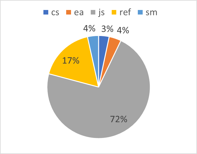
Job sites seem to take a big portion of the funnel, but this isn’t unusual for the Russian market.
As for the analysis itself:
k = relevel(q$pipeline, ref = “js”) #
We’re going to take “job sites” as our reference level, as this is the largest source. All other sources are compared to it.
w1 = coxph(Surv(exp, event) ~ k , data = q)
summary(w1)
Call:
coxph(formula = Surv(exp, event) ~ k, data = q)
n= 1785, number of events= 1004
coef exp(coef) se(coef) z Pr(>|z|)
kcs -0.56725 0.56708 0.19379 -2.927 0.00342 **
kea -0.79360 0.45221 0.19056 -4.165 3.12e-05 ***
kref -0.17166 0.84226 0.08693 -1.975 0.04830 *
ksm -0.25787 0.77269 0.16856 -1.530 0.12605
—
Signif. codes: 0 ‘***’ 0.001 ‘**’ 0.01 ‘*’ 0.05 ‘.’ 0.1 ‘ ’ 1
exp(coef) exp(-coef) lower .95 upper .95
kcs 0.5671 1.763 0.3879 0.8291
kea 0.4522 2.211 0.3113 0.6570
kref 0.8423 1.187 0.7103 0.9987
ksm 0.7727 1.294 0.5553 1.0752
Concordance= 0.542 (se = 0.008 )
Rsquare= 0.018 (max possible= 1 )
Likelihood ratio test= 33.22 on 4 df, p=1.079e-06
Wald test = 28.23 on 4 df, p=1.12e-05
Score (logrank) test = 29.17 on 4 df, p=7.231e-06
To visualize our data, we are going to use the following code:
w = coxph(Surv(exp, event) ~ pipeline , data = q)
summary(w)
plot(survfit(w, newdata=data.frame(pipeline = c(‘cs’, ‘ea’,’js’,
‘ref’, ‘sm’))) ,
xlim = c(0, 12) , ylim = c(0.0, 1),conf.int = FALSE, # Поставьте TRUE
col = c(“red”, “blue”, ‘yellow’, “green”, “grey1”),
lwd = 4, xaxt=’n’, yaxt=’n’)
axis(side=1, at=seq(0, 12, 1), cex.axis=1.5)
axis(side=2, at=seq(0.0 , 1.0, 0.1), las=2, cex.axis=1.5)
abline(v=(seq(0, 12, 1)), col=”black”, lty=”dotted”)
abline(h=(seq(0.0, 1, 0.1)), col=”black”, lty=”dotted”)
legend(“bottomleft”, legend=c(‘cs’, ‘ea’,’js’,
‘ref’, ‘sm’),
col = c(“red”, “blue”, ‘yellow’, “green”, “grey1”), cex = 1.5, lty = 1, pch = “”,
lwd = 4, x.intersp = 0.1, y.intersp = 0.3, text.width = 1, box.lwd = 0)

How should we interpret the results?
Looking at “General Performance”, we can see that this is not very high (Concordance[1]= 0.542). It ranges from 0.5 to 1. In this case, a value of 0.5 indicates no correlation, 1 indicates a full correlation. As such, 0.542 is a very low result. Remember, though, that the result is based on only one variable.
Attrition risk of employees sourced from company career site is 1.76 times lower than employees sourced from job sites (see exp(-coef)).
Employees from employment agencies show 2.2 times lower attrition risk versus employees from job sites.
Employees that were referred also show an attrition risk rate that is 1.18 times lower compared to employees sourced from job sites. The p-value for this finding is 0.048. However, this does not allow us to be sure that referrals have a decreased risk of leaving the company.
Are you surprised by the results? Especially the part concerning referrals? Nowadays, referral programs have a lot of support and are promoted often. However, in our case the referral program does not bring the results we would expect.
Thus, we have our first point of action: Recommend management to analyze the referral program and understand why it doesn’t work as expected. This could be because of a disproportionate referral reward system.
Branches
Let’s take a closer look into turnover in different branches:
summary(q$branch)
fifth first fourth second third
70 541 343 690 141
The names of the branches were removed for confidentiality reasons.

The analysis follows the same pattern as described above and you can easily reproduce it. The results revealed significant differences between branches.
For our next step, we decided to look at the sourced proportions in each branch. An Excel pivot table is a great tool to do this.
Here is a visual representation:

Remember that the 3rd branch has the lowest turnover rate, next is 4th, then 2nd. We found out that branch managers had a lot of freedom in terms of recruitment policy and the graphs above show not only the proportion of recruitment sources, but also the attitude of managers: recruitment through jobsites is low-cost: just post a job and wait for a response. Attraction of personnel in the referral program requires quite some effort. Working with the employment center also takes considerable time, money and effort of the manager/ HR.
Management recommendations:
In conclusion, management is recommended to:
- Analyze the referral program to understand why it does not result in the desired turnover reduction;
- Candidates from the employment agency stayed the longest at the company. So, analyze the candidates from the employment agency and define their “portrait” to use as a reference for recruitment from other sources. For example, as a hypothesis, we could say that candidates from the employment center are of a lower quality;
- Analyze traffic of the company career site and understand why it brings in more candidates to the 3rd branch;
- Allow managers of the 3rd branch to give a workshop on working with employment centers.
[1] Concordance, or C-index, is a metric of survival analysis. This c index, which is derived from the Wilcoxon–Mann–Whitney two-sample rank test, is computed by taking all possible pairs of subjects such that one subject responded and the other did not. The index is the proportion of such pairs with the responder having a higher predicted probability of response than the non-responder. This index equals the difference between the probability of concordance and the probability of discordance of pairs of predicted survival times and pairs of observed survival times, accounting for censoring.
To read more about concordance, check Harrel & Frank’s Regression Modelling Strategies With Applications to Linear Models, Logistic Regression, and Survival Analysis
Weekly update
Stay up-to-date with the latest news, trends, and resources in HR

Learn more
Related articles


Are you ready for the future of HR?
Learn modern and relevant HR skills, online
