Why is knowing about SQL Server storage internals useful? After all, the day-to-day routine of most SQL Server developers and DBAs doesn’t necessarily require detailed knowledge of SQL Server’s inner workings and storage mechanisms. However, armed with it, we will be in a much better position to make optimal design decisions for our systems, and to troubleshoot them effectively when things go wrong and system performance is suffering.

There are so many optimization techniques in a modern RDBMS that we’re unlikely to learn them all. What if, instead of striving to master every technique, we strive to understand the underlying structures that these techniques try to optimize? Suddenly, we have the power of deductive reasoning. While we might not know about every specific feature, we can deduce why they exist as well as how they work. It will also help us to devise effective optimization techniques of our own.

In essence, this is a simple manifestation of the ancient Chinese proverb:

Give a man a fish and you feed him for a day; teach a man to fish and you feed him for a lifetime.

It’s the reason I believe every SQL Server DBA and developer should have a sound basic understanding, not just of what storage objects exist in SQL Server (heaps and indexes), but of the underlying data structures (pages and records) that make up these objects, what they look like at the byte level and how they work. Once we have this, we can make much better decisions about our storage requirements, in terms of capacity, as well as the storage structures we need for optimal query performance.

The Power of Deductive Reasoning

I want to start with a story that explains how I came to appreciate fully the value of knowing what SQL Server actually stores on disk and how. It is also a cautionary tale of how ignorance of the basic underlying structures of the database means that you don’t have the right set of tools to evaluate and design an effective SQL Server solution.

When I first started out with SQL Server, and before I developed any deep knowledge of it, a print magazine retailer asked me to create a system for presenting their magazines online and tracking visitor patterns and statistics. They wanted to know how many views a given magazine page attracted, on an hourly level.

Quick to fetch my calculator, I started crunching the numbers. Assuming each magazine had an average of 50 pages, each page being viewed at least once an hour, this would result in roughly half a million rows (50 pages * 365 days * 24 hours) of data in our statistics table in the database, per year, per magazine. If we were to end up with, say, 1,000 magazines then, well, this was approaching more data than I could think about comfortably and, without any knowledge of how a SQL Server database stored data, I leapt to the conclusion that it would not be able to handle it either.

In a flash of brilliance, an idea struck me. I would split out the data into separate databases! Each magazine would get its own statistics database, enabling me to filter the data just by selecting from the appropriate statistics database, for any given magazine (all of these databases were stored on the same disk; I had no real grasp of the concept of I/O performance at this stage).

I learned my lesson the hard way. Once we reached that magic point of having thousands of magazines, our database backup operations were suffering. Our backup window, originally 15 minutes, expanded to fill 6 hours, simply due to the need to back up thousands of separate databases. The DDL involved in creating databases on the fly as well as creating cross-database queries for comparing statistics…well, let’s just say it wasn’t optimal.

Around this time, I participated in my first SQL Server-oriented conference and attended a Level 200 session on data file internals. It was a revelation and I immediately realized my wrongdoing. Suddenly, I understood why, due to the way data was stored and traversed, SQL Server would easily have been able to handle all of my data. It struck me, in fact, that I’d been trying to replicate the very idea behind a clustered index, just in a horribly inefficient way.

Of course, I already knew about indexes, or so I thought. I knew you created them on some columns to make queries work faster. What I started to understand thanks to this session and subsequent investigations, was how and why a certain index might help and, conversely, why it might not. Most importantly, I learned how b-tree structures allowed SQL Server to efficiently store and query enormous amounts of data.

Records

A record, also known as a row, is the smallest storage structure in a SQL Server data file. Each row in a table is stored as an individual record on disk. Not only table data is stored as records, but also indexes, metadata, database boot structures and so forth. However, we’ll concentrate on only the most common and important record type, namely the data record, which shares the same format as the index record.

Data records are stored in a fixedvar format. The name derives from the fact that there are two basic kinds of data types, fixed length and variable length. As the name implies, fixed-length data types have a static length from which they never deviate. Examples are 4-byte integers, 8-byte datetimes, and 10-byte characters (char(10)).

Variable-length data types, such as varchar(x) and varbinary(x), have a length that varies on a record-by-record basis. While a varchar(10) might take up 10 bytes in one record, it might only take up 3 bytes in another, depending on the stored value.

Figure 1 shows the basic underlying fixedvar structure of every data record.

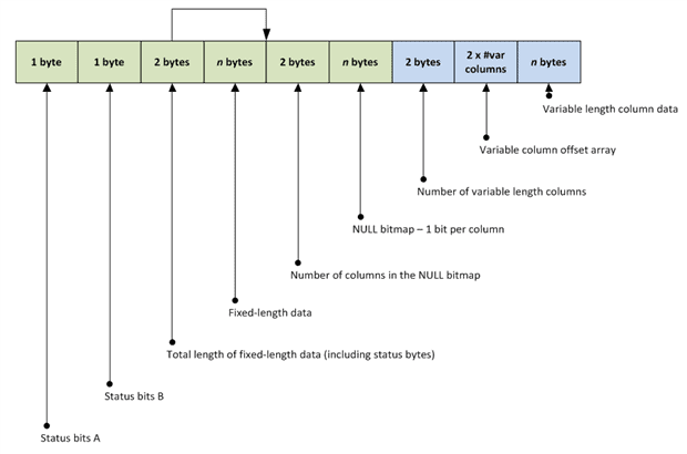
Figure 1: Structure of a data record at the byte level.

Every data record starts with two status bytes, which define, among other things:

• the record type – of which the data and index types are, by far, the most common and important
• whether the record has a null bitmap – one or more bytes used to track whether columns have null values
• whether the record has any variable-length columns.

The next two bytes store the total length of the fixed-length portion of the record. This is the length of the actual fixed-length data, plus the 2 bytes used to store the status, and the 2 bytes used to store the total fixed length. We sometimes refer to the fixed-length length field as the null bitmap pointer, as it points to the end of the fixed-length data, which is where the null bitmap starts.

The fixed-length data portion of the record stores all of the column data for the fixed-length data types in the table schema. The columns are stored in physical order and so can always be located at a specific byte index in the data record, by calculating the size of all the previous fixed-length columns in the schema.

The next two areas of storage make up the null bitmap, an array of bits that keep track of which columns contain null values for that record, and which columns have non-null values in the record. As fixed-length data columns always take up their allotted space, we need the null bitmap to know whether a value is null. For variable-length columns, the null bitmap is the means by which we can distinguish between an empty value and a null value. The 2 bytes preceding the actual bitmap simply store the number of columns tracked by the bitmap. As each column in the bitmap requires a bit, the required bytes for the null bitmap can be calculated by dividing the total number of columns by 8 and then rounding up to the nearest integer: CEIL(#Cols /8).

Finally, we have the variable-length portion of the record, consisting of 2 bytes to store the number of variable-length columns, followed by a variable-length offset array, followed by the actual variable-length data. Figure 2 shows an expanded example of the sections of the data record relating to variable-length data.

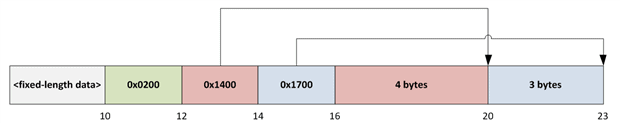
Figure 2: Variable-length data portion of a data record.

We start with two bytes that indicate the number of variable-length columns stored in the record. In this case, the value, 0x0200, indicates two columns. Next up is a series of two-byte values that form the variable-length offset array, one for each column, pointing to the byte index in the record where the related column data ends. Finally, we have the actual variable-length columns.

Since SQL Server knows the data starts after the last entry in the offset array, and knows where the data ends for each column, it can calculate the length of each column, as well as query the data.

Pages

Theoretically, SQL Server could just store a billion records side by side in a huge data file, but that would be a mess to manage. Instead, it organizes and stores records in smaller units of data, known as pages. Pages are also the smallest units of data that SQL Server will cache in memory (handled by the buffer manager).

There are different types of pages; some store data records, some store index records and others store metadata of various sorts. All of them have one thing in common, which is their structure. A page is always exactly 8 KB (8192 bytes) in size and contains two major sections, the header and the body. The header has a fixed size of 96 bytes and has the same contents and format, regardless of the page type. It contains information such as how much space is free in the body, how many records are stored in the body, the object to which the page belongs and, in an index, the pages that precede and succeed it.

The body takes up the remaining 8096 bytes, as depicted in Figure 3.

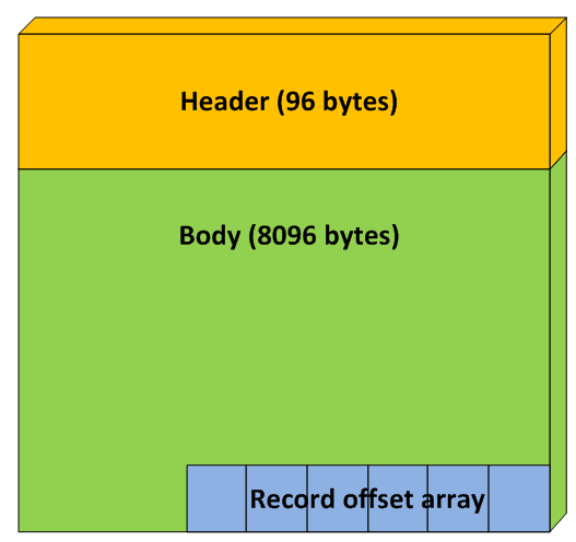
Figure 3: The structure of a page.

At the very end of the body is a section known as the record offset array, which is an array of two-byte values that SQL Server reads in reverse from the very end of the page. The header contains a field that defines the number of slots that are present in the record offset array, and thus how many two-byte values SQL Server can read. Each slot in the record offset array points to a byte index in the page where a record begins. The record offset array dictates the physical order of the records. As such, the very last record on the page, logically, may very well be the first record, physically. Typically, you’ll find that the first slot of the record offset array, stored in the very last two bytes of the page, points to the first record stored at byte index 96, which is at the very beginning of the body, right after the header.

If you’ve ever used any of the DBCC commands, you will have seen record pointers in the format (X:Y:Z), pointing to data file X, page Y and slot Z. To find a record on page Y, SQL Server first needs to find the path for the data file with id X. The file is just one big array of pages, with the very first page starting at byte index 0, the next one at byte index 8192, the third one at byte index 16384, and so on. The page number correlates directly with the byte index, in that page 0 is stored at byte index 0*8192, page 1 is stored at byte index 1*8192, page 2 is stored at byte index 2*8192 and so on. Therefore, to find the contents of page Y, SQL Server needs to read 8192 bytes beginning at byte index Y*8192. Having read the bytes of the page, SQL Server can then read entry Z in the record offset array to find out where the record bytes are stored in the body.

Investigating Page Contents Using DBCC Commands

It’s surprisingly easy to peek into the innards of SQL Server databases, at the bytes that make up your database. We can use one of the three DBCC commands: DBCCTRACEON, DBCCPAGE, and DBCCIND. Microsoft has not officially documented the latter two, but people use them so widely that you can assume that they’re here to stay.

DBCCIND provides the relevant page IDs for any object in the database, and then DBCCPAGE allows us to investigate what’s stored on disk on those specific pages. Note that DBCCPAGE and IND are both ready-only operations, so they’re completely safe to use.

DBCC PAGE

By default, SQL Server sends the output from DBCCPAGE to the trace log and not as a query result. To execute DBCCPAGE commands from SSMS and see the results directly in the query results window, we first need to enable Trace Flag 3604, as shown in Listing 1.

Listing 1: Enabling and disabling Trace Flag 3604.

The trace flag activates at the connection level, so enabling it in one connection will not affect any other connections to the server. Likewise, as soon as the connection closes, the trace flag will no longer have any effect. Having enabled the trace flag, we can issue the DBCCPAGE command using the following syntax:

DBCC PAGE (<Database>, <FileID>, <PageID>, <Style>)

Database is the name of the database whose page we want to examine. Next, the FileIDof the file we want to examine; for most databases this will be 1, as there will only be a single data file. Execute Listing 2 within a specific database to reveal a list of all data files for that database, including their FileIDs.

Listing 2: Interrogating sys.database_files.

Next, the PageID of the page we wish to examine. This can be any valid PageID in the database. For example, the special file header page is page 0, page 9 is the equally special boot page, which is only stored in the primary file with file_id 1, or any other data page that exists in the file. Typically, you won’t see user data pages before page 17+.

Finally, we have the Style value:

• 0 – outputs only the parsed header values. That is, there are no raw bytes, only the header contents.
• 1 – outputs the parsed header as well as the raw bytes of each record on the page.
• 2 – outputs the parsed header as well as the complete raw byte contents of the page, including both the header and body.
• 3 – outputs the parsed header and the parsed record column values for each record on the page. The raw bytes for each record are output as well. This is usually the most useful style as it allows access to the header as well as the ability to correlate the raw record bytes with the column data.

Listing 3 shows how you’d examine the rows on page 16 in the primary data file of the AdventureWorks2008R2 database.

Listing 3: Using DBCCPAGE on AdventureWorks.

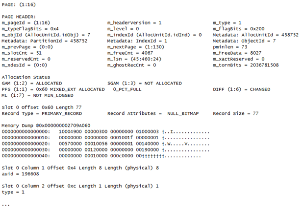Looking at the output, you’ll be able to see the page ID stored in the header (m_pageId), the number of records stored on the page (m_slotCnt), the object ID to which this page belongs (m_objId) and much more.

After the header, we see each record listed, one by one. The output of each record consists of the raw bytes (Memory Dump), followed by each of the column values (Slot0Column1..., and so on). Note that the column values also detail how many (physical) bytes they take up on disk, making it easier for you to correlate the value with the raw byte output.

DBCC IND

Now that you know how to gain access to the contents of a page, you’ll probably want to do so for tables in your existing databases. What we need, then, is to know on which pages a given table’s records are stored. Luckily, that’s just what DBCCIND provides and we call it like this:

We specify the name of the database and the name of the object for which we wish to view the pages. Finally, we can filter the output to just a certain index; 0 indicates a heap, while 1 is the clustered index. If we want to see the pages for a specific non-clustered index, we enter that index’s ID. If we use -1 for the IndexID, we get a list of all pages belonging to any index related to the specified object.

Listing 4 examines the Person.Person table in the SQL Server 2008 R2 AdventureWorks database, and is followed by the first five rows of the results (your output may differ, depending on the release).

Listing 4: Using DBCCIND on AdventureWorks.

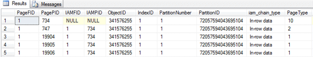
There are a couple of interesting columns here. The PageType column details the type of page. For example, PageType 10 is an allocation structure page known as an IAM page, which I’ll describe in the next section. PageType 2 is an index page and PageType 1 is a data page.

The first two columns show the file ID as well as the page ID of each of those pages. Using those two values, we can invoke DBCCPAGE for the first data page, as shown in Listing 5.

Listing 5: Using DBCCPAGE to view the contents of a data page belonging to the Person.Person table.

Heaps and Indexes

We’ve examined the structure of records and the pages in which SQL Server stores them. Now it’s time for us to go a level higher, and look at how SQL Server structures pages in heaps and indexes. If a table contains a clustered index, then that table is stored in the same way as an index. A table without a clustered index is a “heap.”

Heaps

Heaps are the simplest data structures, in that they’re just “a big bunch of pages,” all owned by the same object. A special type of page called an index allocation map (IAM) tracks which pages belong to which object. SQL Server uses IAM pages for heaps and indexes, but they’re especially important for heaps as they’re the only mechanism for finding the pages containing the heap data. My primary goal in this article is to discuss index structure and design, so I’ll only cover heaps briefly.

Each IAM page contains one huge bitmap, tracking 511,232 pages, or about 4 GB of data. For the sake of efficiency, the IAM page doesn’t track the individual pages, but rather groups of eight, known as extents. If the heap takes up more than 4 GB of data, SQL Server allocates another IAM page to enable tracking the pages in the next 4 GB of data, leaving in the first IAM page’s header a pointer to the next IAM page. In order to scan a heap, SQL Server will simply find the first IAM page and then scan each page in each extent to which it points.

One important fact to remember is that a heap guarantees no order for the records within each page. SQL Server inserts a new record wherever it wants, usually on an existing page with plenty of space, or on a newly allocated page.

Compared to indexes, heaps are rather simple in terms of maintenance, as there is no physical order to maintain. We don’t have to consider factors such as the use of an ever-increasing key for maintaining order as we insert rows; SQL Server will just append a record anywhere it fits, on its chosen page, regardless of the key.

However, just because heap maintenance is limited, it doesn’t mean that heaps have no maintenance issues. In order to understand why, we need to discuss forwarded records.

Unlike in an index, a heap has no key that uniquely identifies a given record. If a non-clustered index or a foreign key needs to point to a specific record, it does so using a pointer to its physical location, represented as (FileID:PageID:SlotID), also known as a RID or a row identifier. For example (1:16:2) points to the third slot in the 17th page (both starting at index 0) in the first file (which starts at index 1).

Imagine that the pointer to record (1:16:2) exists in 20 different places but that, due perhaps to an update to a column value, SQL Server has to move the record from page 16 as there is no longer space for it. This presents an interesting performance problem.

If SQL Server simply moves the record to a new physical location, it will have to update that physical pointer in 20 different locations, which is a lot of work. Instead, it copies the record to a new page and converts the original record into a forwarding stub, a small record taking up just 9 bytes storing a physical pointer to the new record. The existing 20 physical pointers will read the forwarding stub, allowing SQL Server to find the wanted data.

This technique makes updates simpler and faster, at the considerable cost of an extra lookup for reads. As data modifications lead to more and more forwarded records, disk I/O increases tremendously, as SQL Server tries to read records from all over the disk.

Listing 6 shows how to query the sys.dm_db_index_physical_stats DMV to find all heaps with forwarded records in the AdventureWorks database. If you do have any heaps (hopefully not), then monitor these values to decide when it’s time to issue an ALTERTABLEREBUILD command to remove the forwarded records.

Listing 6: Using sys.dm_db_index_physical_stats to monitor the number of forwarded records in any heaps in a database.

Indexes

SQL Server also tracks which pages belong to which indexes through the IAM pages. However, indexes are fundamentally different from heaps in terms of their organization and structure. Indexes, clustered as well as non-clustered, store data pages in a guaranteed logical order, according to the defined index key (physically, SQL Server may store the pages out of order).

Structurally, non-clustered and clustered indexes are the same. Both store index pages in a structure known as a b-tree. However, while a non-clustered index stores only the b-tree structure with the index key values and pointers to the data rows, a clustered index stores both the b-tree, with the keys, and the actual row data at the leaf level of the b-tree. As such, each table can have only one clustered index, since the data can only be stored in one location, but many non-clustered indexes that point to the base data. With non-clustered indexes, we can include copies of the data for certain columns, for example so that we can read frequently accessed columns without touching the base data, while either ignoring the remaining columns or following the index pointer to where the rest of the data is stored.

For non-clustered indexes, the pointer to the actual data may take two forms. If we create the non-clustered index on a heap, the only way to locate a record is by its physical location. This means the non-clustered index will store the pointer in the form of an 8-byte row identifier. On the other hand, if we create the non-clustered index on a clustered index, the pointer is actually a copy of the clustered key, allowing us to look up the actual data in the clustered index. If the clustered key contains columns already part of the non-clustered index key, those are not duplicated, as they’re already stored as part of the non-clustered index key.

Let’s explore b-trees in more detail.

b-tree structure

The b-tree structure is a tree of pages, usually visualized as an upside-down tree, starting at the top, from the root, branching out into intermediate levels, and finally ending up at the bottom level, the leaf level. If all the records of an index fit on one page, the tree only has one level and so the root and leaf level can technically be the same level. As soon as the index needs two pages, the tree will split up into a root page pointing to two child pages at the leaf level. For clustered indexes, the leaf level is where SQL Server stores all the data; all the intermediate (that is, non-leaf) levels of the tree contain just the data from the key columns. The smaller the key, the more records can fit on those branch pages, thus resulting in a shallower tree depth and quicker leaf lookup speed.

The b-tree for an index with an integer as the index key might look something like the one shown in Figure 4.

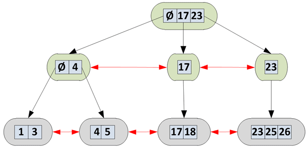
Figure 4: A b-tree structure for an index with an integer key.

The bottom level is the leaf level, and the two levels above it are branches, with the top level containing the root page of the index (of which there can be only one). In this example, I’m only showing the key values, and not the actual data itself, which would otherwise be in the bottom leaf level, for a clustered index. Note that the leftmost intermediate level pages will always have an à entry. It represents any value lower than the key next to it. In this case, the root page à covers values 1-16 while the intermediate page à covers the values 1-3.

The main point to note here is that the pages connect in multiple ways. On each level, each page points to the previous and the next pages, provided these exist, and so acts as a doubly-linked list. Each parent page contains pointers to the child pages on the level below, all the way down to the leaf level, where there are no longer any child page pointers, but actual data, or pointers to the actual data, in the case of a non-clustered index.

If SQL Server wants to scan a b-tree, it just needs a pointer to the root page. SQL Server stores this pointer in the internal sys.sysallocunits base table, which also contains a pointer to the first IAM page tracking the pages belonging to a given object. From the root page, it can follow the child pointers all the way until the first leaf-level page, and then just scan the linked list of pages.

The power of b-trees: binary searches, a.k.a. seeking

You’ve probably heard the age-old adage that scans are bad and seeks are good, and with good reason because, in general, these are wise words.

As discussed previously, in a heap there is no order to the data, so if SQL Server wants to find a specific value, it can only do so by scanning all of the data in the heap. Even if we run a “SELECTTOP1” query, SQL Server may still need to scan the entire table to return just that single row, if the first row of the result set happens to be the very the last record in the heap. Of course, if we happen to have a non-clustered index on the heap that includes the required columns, SQL Server may perform a seek operation.

Conversely, finding a specific value in a b-tree is extremely efficient. By exploiting the fact that the b-tree logically sorts all of the values by index key, we can use an algorithm called binary search to find the desired value in very few operations.

Imagine a game where Player A thinks of a number between 1 and 10 that Player B has to guess. On each guess from Player B, Player A must only offer one of three replies: “correct,” “lower” or “higher.”

Player A thinks of a number. Player B, a wise opponent, asks if the number is “5.” Player B responds “higher,” so B now knows that the number is 6, 7, 8, 9, or 10. Aiming for the middle of the set again, B guesses “8.” A responds “higher” so now B knows it’s either 9 or 10. B guesses “9” and A responds with “correct.” By always going for the median value, Player B cut the number of values in half on each guess, narrowing down the possible values very quickly.

SQL Server uses similar logic to traverse the b-tree to find a specific value. Let’s say SQL Server, in response to a query, needs to find the record corresponding to Key 5, in Figure 4. First, it looks at the middle key on the root page, 17, indicating that the page to which it points contains values of 17 and higher. Five is smaller than 17 so it inspects the middle key of all the keys lower than 17. In this simple example, there is only the à key so it follows this link to the page in the next level and inspects the value of the middle key. As there are only two keys, it will round up, look at the rightmost key, holding the value 4, and follow the chain to the leaf-level page containing Keys 4 and 5, at which point it has found the desired key.

If, instead, the search is for the Key 22, SQL Server starts in the same way but this time, after 17, inspects the middle key of all the keys higher than 17. Finding only Key 23, which is too high, it concludes that the page to which Key 17 points in the second level contains the values 17-22. From here, it follows the only available key to the leaf level, is unable to find the value 22 and concludes that no rows match the search criteria.

The downside to b-trees: maintenance

Though they enable efficient seeking, b-trees come with a price. SQL Server has to ensure that the records remain sorted in the correct key order at all times. In Figure 5, on the left we have a very small tree, with just an integer as the key. It contains two levels, consisting of a root page with two child pages. We’ll assume that each of the leaf-level pages contains a lot of data besides just the keys, so can’t hold more than two records. If we want to insert the value 15, SQL Server has to introduce a third leaf page. It can’t just add the new row on a third page at the end, as it must insert the value 15 between 10 and 20. The result is a page split. SQL Server simply takes the existing page, containing the values 10 and 20, and splits it into two pages, storing half the rows on the new page, and half of them on the original page. There is now enough space for SQL Server to insert the value 15 on the half-empty original page, containing the value 10.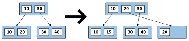

Figure 5: A page split.

After splitting the page, we now have three pages in the leaf level and three keys in the root page. The page split is a costly operation for SQL Server in its own right, compared to simply inserting a record on an existing page, but the real cost is paid in terms of the fragmentation that arises from splitting pages. We no longer have a physically contiguous list of pages; SQL Server might store the newly allocated page in an entirely different area of disk. As a result, when we scan the tree, we’ll have to read the first page, potentially skip to a completely different part of the disk, and then back again to continue reading the pages in order.

As time progresses and fragmentation gets worse, you’ll see performance slowly degrading. Insertions will most likely run at a linear pace, but scanning and seeking will get progressively slower.

An easy way to avoid this problem is to avoid inserting new rows between existing ones. If we use an ever-increasing identity value as the key, we always add rows to the end, and SQL Server will never have to split existing pages. If we delete existing rows we will still end up with half-full pages, but we will avoid having the pages stored non-contiguously on disk.

Crunching the Numbers

Based on this understanding of the underlying structure of data records and pages and indexes, how might I have made better design and capacity planning choices for the magazine statistics database? Listing 7 shows a basic schema for the new design.

Listing 7: New schema design for the MagazineStatistics table.

It is surprisingly simple. Part of the beauty here was in designing a schema that doesn’t need any secondary indexes, just the clustered index. In essence, I’d designed a single clustered index that served the same purpose as my thousands of separate databases, but did so infinitely more efficiently.

Index design

There’s one extremely high-impact choice we have to make up front, namely, how to design the clustered index, with particular regard to the ViewDate column, an ever-increasing value that tracks the date and hour of the page view. If that’s the first column of the clustered index, we’ll vastly reduce the number of page splits, since SQL Server will simply add each new record to the end of the b-tree. However, in doing so, we’ll reduce our ability to filter results quickly, according MagazineID. To do so, we’d have to scan all of the data.

I took into consideration that the most typical query pattern would be something like “Give me the total number of page views for magazine X in the period Y.” With such a read pattern, the schema in Listing 7 is optimal since it sorts the data by MagazineID and ViewDate.

While the schema is optimal for reading, it’s suboptimal for writing, since SQL Server cannot write data contiguously if the index sorts by MagazineID first, rather than by ViewDate column. However, within each MagazineID, SQL Server will store the records in sorted order thanks to the ViewDate and ViewHour columns being part of the clustered key.

This design will still incur a page split cost as we add new records but, as long as we perform regular maintenance, old values will remain unaffected. By including the PageNumber column as the fourth and last column of the index key, it is also relatively cheap to satisfy queries like “Give me the number of page views for page X in magazine Y in period Z.”

While you would generally want to keep your clustered key as narrow as possible, it’s not necessary in this case. The four columns in the key only add up to 9 bytes in total, so it’s still a relatively narrow key compared, for example, to a 16-byte uniqueidentifier (GUID).

The presence of non-clustered indexes or foreign keys in related tables exacerbates the issue of a wide clustering key, due to the need to duplicate the complete clustered key. Given our schema and query requirements, we had no need for non-clustered indexes, nor did we have any foreign keys pointing to our statistics data.

Storage requirements

The MagazineStatistics table has two 4-byte integers, a 2-byte smallint, a 4-byte smalldatetime and a 1-byte tinyint. In total, that’s 11 bytes of fixed-length data. To calculate the total record size, we need to add the two status bytes, the two fixed-length length bytes, the two bytes for the null bitmap length indicator, as well as a single byte for the null bitmap itself. As there are no variable-length columns, the variable-length section of the record won’t be present. Finally, we also need to take into account the two bytes in the record offset array at the end of the page body (see Figure 3). In total, this gives us a record size of 20 bytes per record. With a body size of 8096 bytes, that enables us to store 8096 / 20 = 404 records per page (known as the fan-out).

Assuming each magazine had visitors 24/7, and an average of 50 pages, that gives us 365 * 24 * 50 = 438,000 records per magazine, per year. With a fan-out of 404, that would require 438,000 / 404 = 1,085 data pages per magazine, weighing in at 1,085 * 8 KB = 8.5 MB in total. As we can’t keep the data perfectly defragmented (as the latest added data will suffer from page splits), let’s add 20% on top of that number just to be safe, giving a total of 8.5 + 20% = 10.2 MB of data per magazine per year. If we expect a thousand magazines per year, all with 24/7 traffic on all pages, that comes in at just about 1,000 * 10.2 MB = 9.96 GB of data per year.

In reality, the magazines don’t receive traffic 24/7, especially not on all pages. As such, the actual data usage is lower, but these were my “worst-case scenario” calculations.

Summary

I started out having no idea how to calculate the required storage with any degree of accuracy, no idea how to create a suitable schema and index key, and no idea of how SQL Server would manage to navigate my data. That one session on SQL Server Internals piqued my interest in understanding more and, from that day on, I realized the value in knowing what happens internally and how I could use that knowledge to my advantage.

If this article has piqued your interest too, I strongly suggest you pick up Microsoft SQL Server 2008 Internals by Kalen Delaney et al., and drill further into the details.

SQL Server Storage Internals 101 is an excerpt from Tribal SQL, a community book featuring 15 authors for 15 chapters. For more information about the book and how to get your copy, please visit www.TribalSQL.com.