Production Deep Learning with NVIDIA GPU Inference Engine

[Update September 13, 2016: GPU Inference Engine is now TensorRT]

Today at ICML 2016, NVIDIA announced its latest Deep Learning SDK updates, including DIGITS 4, cuDNN 5.1 (CUDA Deep Neural Network Library) and the new GPU Inference Engine.

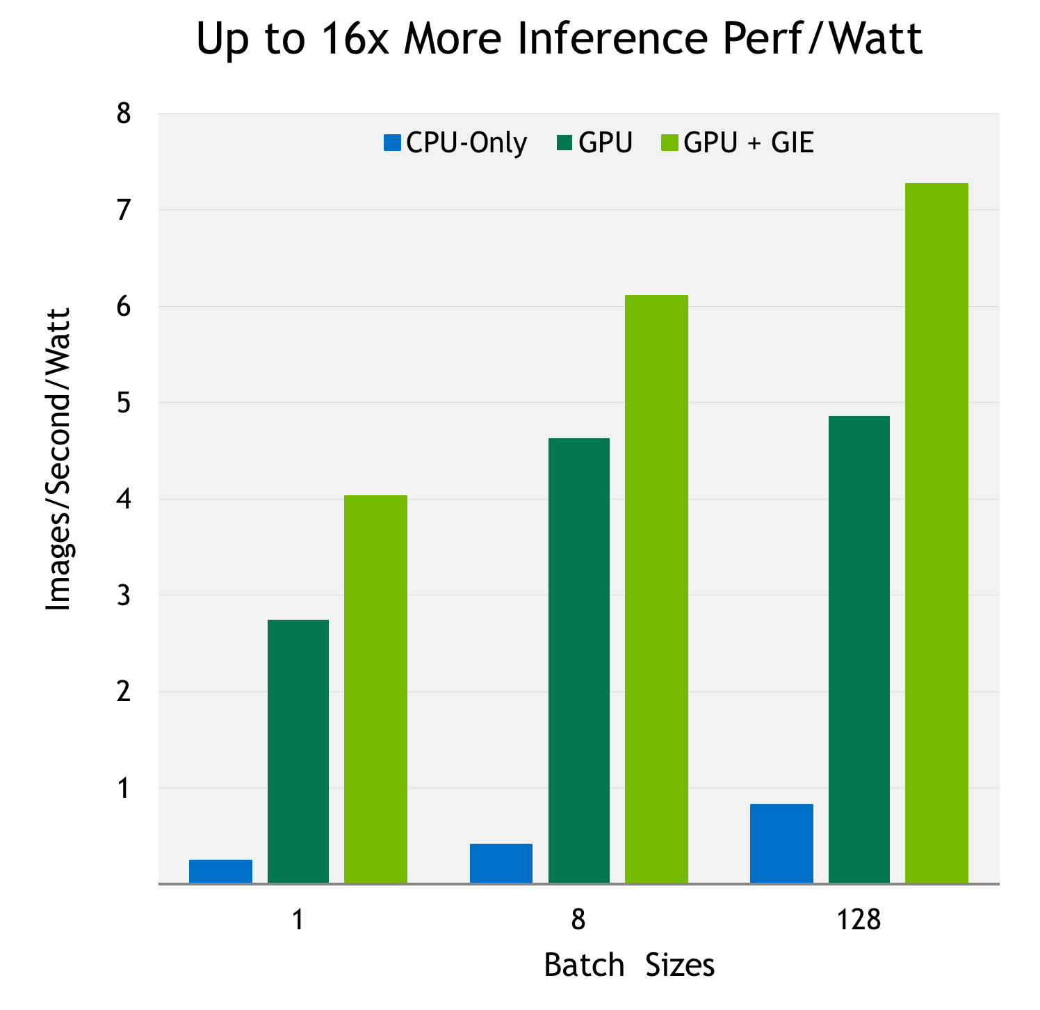
NVIDIA GPU Inference Engine (GIE) is a high-performance deep learning inference solution for production environments. Power efficiency and speed of response are two key metrics for deployed deep learning applications, because they directly affect the user experience and the cost of the service provided. GIE automatically optimizes trained neural networks for run-time performance, delivering up to 16x higher performance per watt on a Tesla M4 GPU compared to the CPU-only systems commonly used for inference  today.

Figure 1 shows GIE inference performance per watt of the relatively complex GoogLeNet running on a Tesla M4. GIE can deliver 20 Images/s/Watt on the simpler AlexNet benchmark.

In this post, we will discuss how you can use GIE to get the best efficiency and performance out of your trained deep neural network on a GPU-based deployment platform.

Deep Learning Training and Deployment

Solving a supervised machine learning problem with deep neural networks involves a two-step process.

1. The first step is to train a deep neural network on massive amounts of labeled data using GPUs. During this step, the neural network learns millions of weights or parameters that enable it to map input data examples to correct responses. Training requires iterative forward and backward passes through the network as the objective function is minimized with respect to the network weights. Often several models are trained and accuracy is validated against data not seen during training in order to estimate real-world performance.
2. The next step–inference–uses the trained model to make predictions from new data. During this step, the best trained model is used in an application running in a production environment such as a data center, an automobile, or an embedded platform. For some applications, such as autonomous driving, inference is done in real time and therefore high throughput is critical.

To learn more about the differences between training and inference, see Michael Andersch’s post on inference with GPUs.

The target deployment environment introduces various challenges that are typically not present in the training environment. For example, if the target is an embedded device using the trained neural network to perceive its surroundings, then the forward inference pass through the model has a direct impact on the overall response time and the power consumed by the device.  The key metric to optimize is power efficiency: the inference performance per watt.

Performance per watt is also the critical metric in maximizing data center operational efficiency.  In this scenario, the need to minimize latency and energy used on large volumes of geographically and temporally disparate requests limits the ability to form large batches.

Introducing GPU Inference Engine

GIE is a high-performance inference engine designed to deliver maximum inference throughput and efficiency for common deep learning applications such as image classification, segmentation, and object detection. GIE optimizes your trained neural networks for run-time performance and delivers GPU-accelerated inference for web/mobile, embedded and automotive applications.

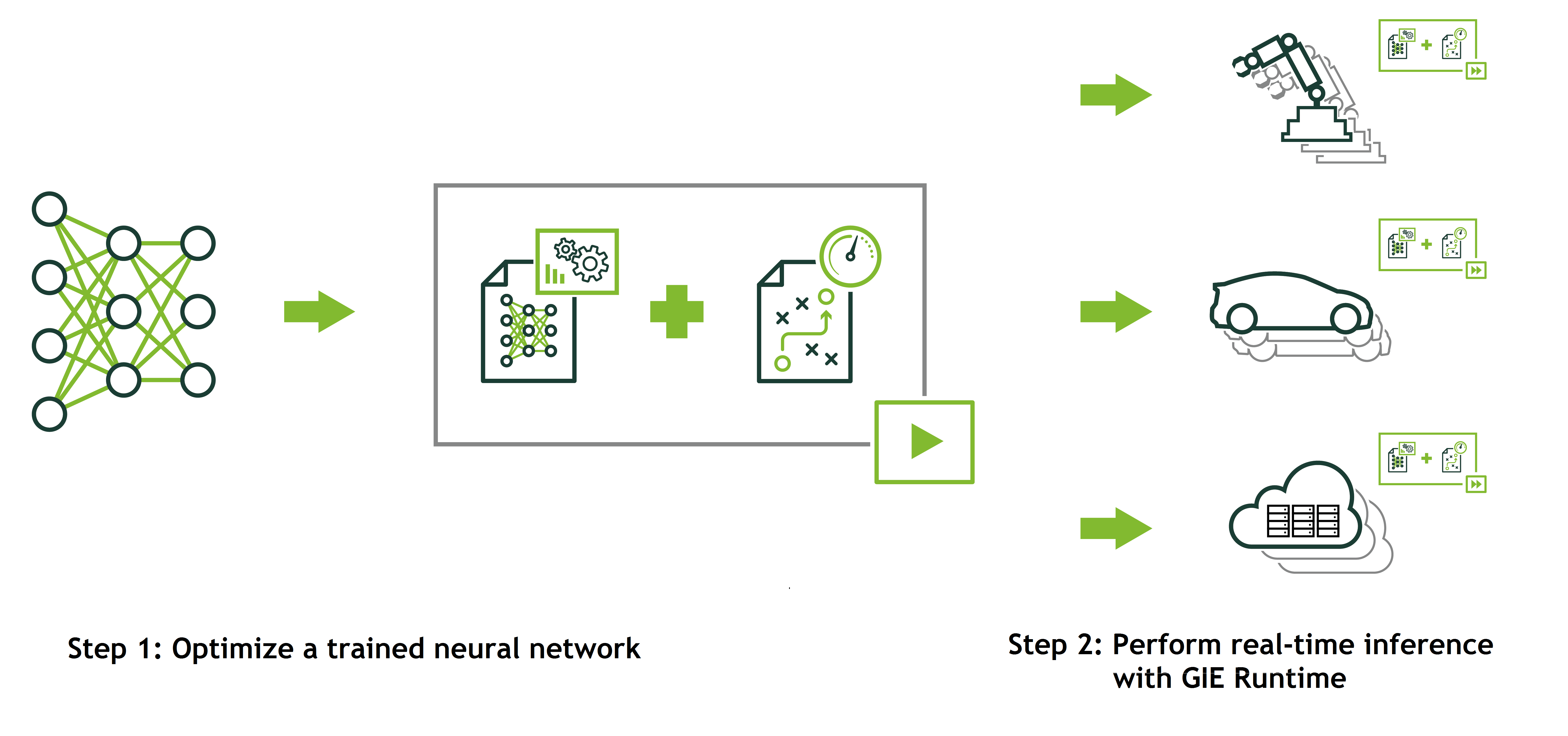
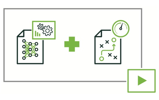
There are two phases in the use of GIE: build and deployment (See Figure 2). In the build phase, GIE performs optimizations on the network configuration and generates an optimized plan for computing the forward pass through the deep neural network. The plan is an optimized object code that can be serialized and stored in memory or on disk.

The deployment phase generally takes the form of a long running service or user application that accepts batches of input data, performs inference by executing the plan on the input data and returns batches of output data (classification, object detection, etc). With GIE you don’t need to install and run a deep learning framework on the deployment hardware. Discussion of the batching and pipeline of the inference service is a topic for another post; instead we will focus on how to use GIE for inference.

GIE Build Phase

The GIE runtime needs three files to deploy a classification neural network:

1. a network architecture file (deploy.prototxt),
2. trained weights (net.caffemodel), and
3. a label file to provide a name for each output class.

In addition, you must define the batch size and the output layer. Code Listing 1 illustrates how to convert a Caffe model to a GIE object. The builder (lines 4-7) is responsible for reading the network information. Alternatively, you can use the builder to define the network information if you don’t provide a network architecture file (deploy.prototxt).

GIE supports the following layer types.

• Convolution: 2D
• Activation: ReLU, tanh and sigmoid
• Pooling: max and average
• ElementWise: sum, product or max of two tensors
• LRN: cross-channel only
• Fully-connected: with or without bias
• SoftMax: cross-channel only
• Deconvolution

IBuilder* builder = createInferBuilder(gLogger);

// parse the caffe model to populate the network, then set the outputs
INetworkDefinition* network = builder->createNetwork();

CaffeParser parser;
auto blob_name_to_tensor = parser.parse(“deploy.prototxt”,
                                        trained_file.c_str(),
                                        *network,
                                        DataType::kFLOAT);

// specify which tensors are outputs
network->markOutput(*blob_name_to_tensor->find("prob"));

// Build the engine
builder->setMaxBatchSize(1);
builder->setMaxWorkspaceSize(1 << 30); 
ICudaEngine* engine = builder->buildCudaEngine(*network);

You can also use the GIE C++ API to define the network without the Caffe parser, as Listing 2 shows. You can use the API to define any supported layer and its parameters. You can define any parameter that varies between networks, including convolution layer weight dimensions and outputs as well as the window size and stride for pooling layers.

ITensor* in = network->addInput(“input”, DataType::kFloat, Dims3{…});
IPoolingLayer* pool = network->addPooling(in, PoolingType::kMAX, …);

After defining or loading the network, you must specify the output tensors as line 13 of Listing 1 shows; in our example the output is “prob” (for probability). Next, define the batch size (line 16), which can vary depending on the deployment scenario. Listing 1 uses a batch size of 1 but you may choose larger batch sizes to fit your application needs and system configuration. Underneath, GIE performs layer optimizations to reduce inference time. While this is transparent to the API user, analyzing the network layers requires memory, so you must specify the maximum workspace size (line 17).

The last step is to call buildCudaEngine to perform layer optimization and build the engine with the optimized network based on your provided inputs and parameters. Once the model is converted to a GIE object it is deployable and can either be used on the host device or saved and used elsewhere.

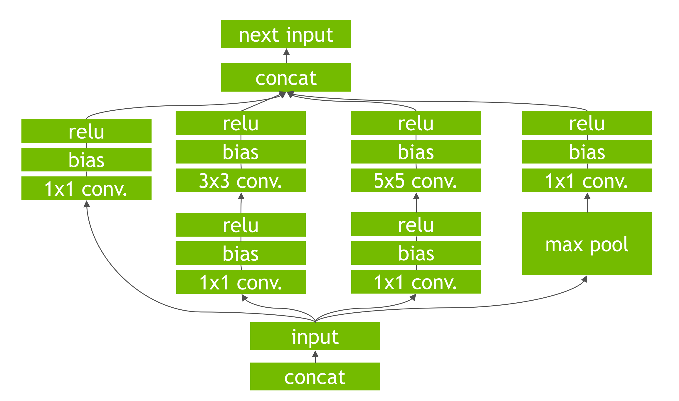
GIE performs several important transformations and optimizations to the neural network graph. First, layers with unused output are eliminated to avoid unnecessary computation. Next, where possible convolution, bias, and ReLU layers are fused to form a single layer. Figure 4 shows the result of this vertical layer fusion on the original network from Figure 3 (fused layers are labeled CBR in Figure 4). Layer fusion improves the efficiency of running GIE-optimized networks on the GPU.

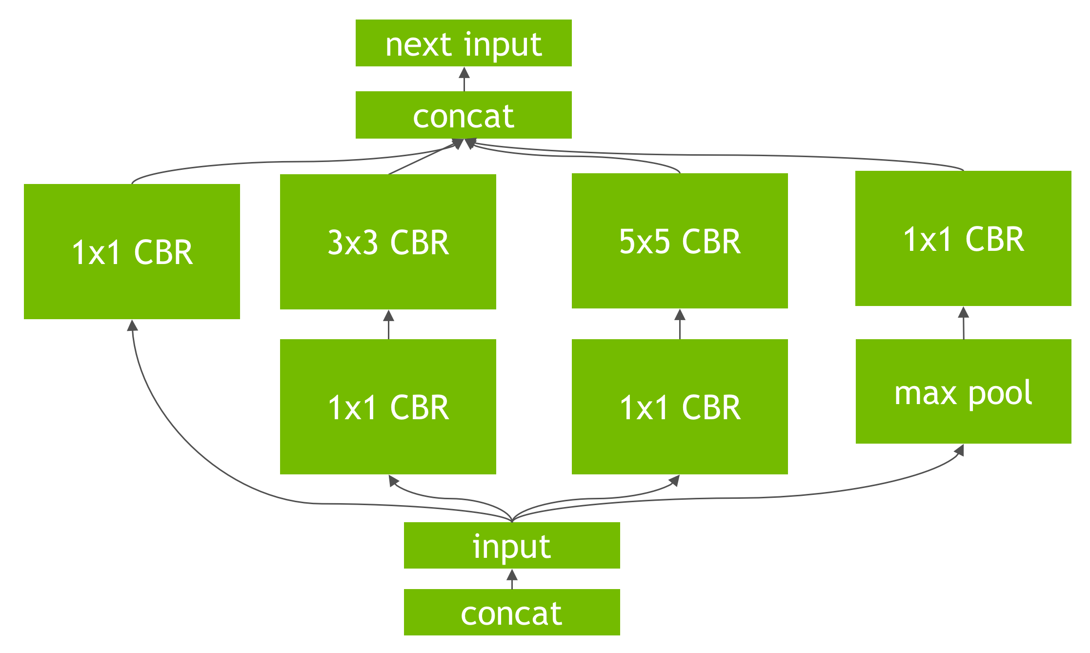
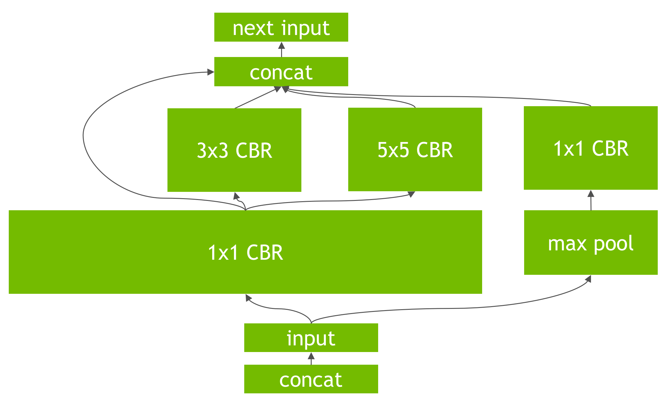
Another transformation is horizontal layer fusion, or layer aggregation, along with the required division of aggregated layers to their respective outputs, as Figure 5 shows. Horizontal layer fusion improves performance by combining layers that take the same source tensor and apply the same operations with similar parameters, resulting in a single larger layer for higher computational efficiency. The example in Figure 5 shows the combination of 3 1×1 CBR layers from Figure 4 that take the same input into a single larger 1×1 CBR layer. Note that the output of this layer must be disaggregated to feed into the different subsequent layers from the original input graph.

GIE performs its transformations during the build phase transparently to the API user after the GIE parser reads in the trained network and configuration file, as Listing 1 shows.

GIE Deploy Phase

The inference builder (IBuilder) buildCudaEngine method returns a pointer to a new inference engine runtime object (ICudaEngine).  This runtime object is ready for immediate use; alternatively, its state can be serialized and saved to disk or to an object store for distribution. The serialized object code is called the Plan.

As mentioned earlier, the full scope of batching and streaming data to and from the runtime inference engine is beyond the scope of this article.  Listing 3 demonstrates the steps required to use the inference engine to process a batch of input data to generate a result.

// The execution context is responsible for launching the 
// compute kernels
IExecutionContext *context = engine->createExecutionContext();

// In order to bind the buffers, we need to know the names of the 
// input and output tensors.
int inputIndex = engine->getBindingIndex(INPUT_LAYER_NAME),
int outputIndex = engine->getBindingIndex(OUTPUT_LAYER_NAME);

// Allocate GPU memory for Input / Output data
void* buffers = malloc(engine->getNbBindings() * sizeof(void*));
cudaMalloc(&buffers[inputIndex], batchSize * size_of_single_input);
cudaMalloc(&buffers[outputIndex], batchSize * size_of_single_output);

// Use CUDA streams to manage the concurrency of copying and executing
cudaStream_t stream;
cudaStreamCreate(&stream);

// Copy Input Data to the GPU
cudaMemcpyAsync(buffers[inputIndex], input, 
                batchSize * size_of_single_input, 
                cudaMemcpyHostToDevice, stream);

// Launch an instance of the GIE compute kernel
context.enqueue(batchSize, buffers, stream, nullptr);

// Copy Output Data to the Host
cudaMemcpyAsync(output, buffers[outputIndex], 
                batchSize * size_of_single_output, 
                cudaMemcpyDeviceToHost, stream));

// It is possible to have multiple instances of the code above
// in flight on the GPU in different streams.
// The host can then sync on a given stream and use the results
cudaStreamSynchronize(stream);

GIE Performance

At the end of the day, the success of GIE comes down to the performance it provides for inference. To measure the performance benefits we compared the per-layer timings of the GoogLeNet network using Caffe and GIE on NVIDIA Tesla M4 GPUs with a batch size of 1 averaged over 1000 iterations with GPU clocks fixed in the P0 state.

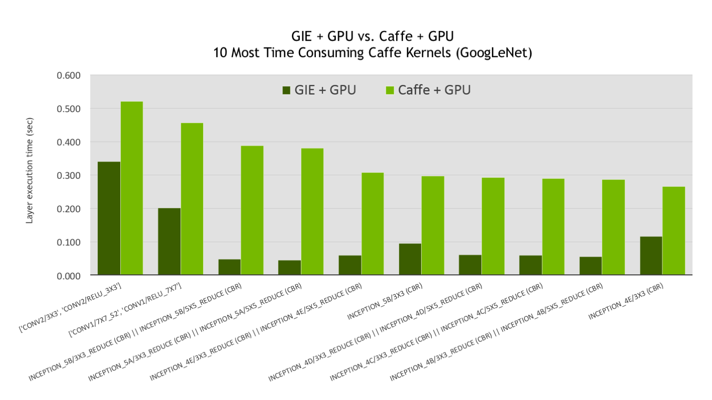
The bar graph (Figure 6) is sorted to show the 10 most computationally expensive GoogLeNet layers (as run by Caffe) ordered from left to right as light green bars. The dark green bars represent the same layers run using GIE (lower is better). Since GIE can combine layers both vertically and horizontally into a single optimized kernel, the Caffe timing shown for each bar is the sum of Caffe kernels corresponding to each fused GIE kernel, while the GIE timing for each bar is for a single fused and optimized kernel.

Bars with two layers correspond to vertically fused layers, namely CBR (convolution + bias + activation/relu). Bars with four layers (or whose names contain “||” separating two CBR layer names) correspond to two CBRs that are horizontally fused, meaning two CBRs that share the same input tensor and thus gain the advantage of cache reuse on a single-pass of the input tensor vs. two separate kernel launches with the same input tensor. Unsurprisingly, the GIE kernels with four fused layers show some of the largest relative speedups and contribute to ~30% of the overall speedup.  The remainder of the speedup predominately comes from the two vertically fused CBR layers, which on average have a lower relative speedup, but comprise the bulk of the computation.

Maximize Performance and Efficiency with GIE

The NVIDIA GPU Inference Engine enables you to easily deploy neural networks to add deep learning based capabilities to your products with the highest performance and efficiency. GIE supports networks trained using popular neural network frameworks including Caffe, Theano, Torch and Tensorflow. During the build phase GIE identifies opportunities to optimize the network, and in the deployment phase GIE runs the optimized network in a way that minimizes latency and maximizes throughput.

If you are running web or mobile applications that are backed by data center servers, GIE’s low overhead means that you can deploy more varied and complex models to add intelligence to your product that will delight your users. If you are using deep learning to create the next generation of smart devices, GIE helps you deploy networks with high performance, high accuracy, and high energy efficiency.

Moreover, GIE enables you to leverage the power of GPUs to perform neural network inference using mixed-precision FP16 data. Performing neural network inference using FP16 can reduce memory usage by half and provide higher performance on Tesla P100 and Jetson TX1 GPUs.

GIE is currently being evaluated under an Early Access (EA) Program. To be notified when GIE is ready for public release or if you are interested in participating in the EA program, please visit the GIE product page to contact us today. To learn more about neural network inference on GPUs, see Michael Andersch’s post on inference with GPUs.